Slip and No Slip Conditions in Serpentine Channel for Bingham Fluid-Numerical CFD Investigation

Kuldeep Panwar

General Electric Power, Noida, India
E-mail: drkuldeep.panwar@sce.org.in

Received 07 January 2022; Accepted 17 February 2022; Publication 04 March 2023

Abstract

For the flow of a Bing-ham fluid in a serpentine tube with a circular cross section, a numerical examination of slip and no slip scenarios was conducted. This was done in order to better understand the flow. This investigation was carried out. In order to get a deeper comprehension of the flow behavior, several flow situations, including slip and no slip, are investigated using separate sets of parameters. In order to solve the issue presented by the turbulent model, the K-model is put to use. It was discovered that the parameter variation for no slip circumstances is preferable to that of no slip scenarios under high stress. This was discovered by comparing the two. A limited analysis of the flow behavior of the Bingham fluid in a serpentine cannel served as the impetus for the current work. The research that was done was motivated by this analysis.

Keywords: Serpentine channel, CFD, non-newtonian channel, slip and no slip.

1 Introduction

The investigation of the flow properties of a viscous fluid in a curved tube is a fundamentally fascinating problem in the field of internal fluid mechanics, which studies the behavior of fluids within restricted spaces. This problem focuses on the properties of the flow of the fluid. A variant of the serpentine tube designs that are commonly used in industrial environments such as heat engines, heat exchangers, and chemical reactors. This variant of the serpentine tube design was developed specifically for use in industrial settings. It is crucial to have an understanding of secondary flow as well as the complex flow field. One form of non-Newtonian fluid known as Bingham fluid is characterized by the presence of a yield strength that, in order for the fluid to flow, must first be overcome. When subjected to mild stresses, a Bingham plastic behaves like a rigid body, but when subjected to high loads, it flows like a viscous fluid.

Bigyani Das [1] demonstrated the flow of a Bingham fluid using the Runga-Kutta Merson Technique by passing the fluid through a very small tube that had a curve in it. During the course of this investigation, the region of the Dean number that was being researched was analyzed, and the results were compared to Casson fluid and found to have the same yield value. By utilizing a curved tube ci, one is able to arrive at the following conclusion on the flow parameters of a Bingham fluid.

Yildiz Bayazitoglu et al. [2] have carried out work of a comparable nature for laminar Bingham fluids that flow between vertical parallel plates. Within the scope of their investigation, it is assumed that the flow of the fluid is laminar, and they provide a reference case for the solution that assumes the flow of viscous fluid is linear. The issue with the Bing-Ham fluid’s natural convection may be explained by the five distinct locations that are present in the space that exists between the parallel plates, starting with the hotter plates and working your way down to the cooler ones. The conclusion that can be drawn from this is that it will make it possible to build designer fluid and tie the thermal performance of fluid to laboratory features. According to the Bingham material model, a change in the behavior of the flow will occur as a direct consequence of the degradation of the gel’s strength caused by the flow.

Fusi et al. [3] As an additional way for researching the fluid, you may run Bingham fluid via a channel that has a pressure-driven lubricating flow. In order to successfully model the lubricating flow of a Bingham fluid through a channel with non-uniform amplitude, it was necessary to make use of this technique. In the end, the technique produces an equation for the integral-differential pressure that can be solved by an iterative procedure. Additionally, the scope of the research is broadened to address the question of how pressure affects viscosity. Research was carried out by Mukherjee and colleagues to investigate the impact that the Bingham plastic viscosity and power law have on the flow and features of heat transfer laminar forced convection in non-circular ducts. The researchers were interested in how these factors influence the heat transfer. Two different thermal boundary conditions have been developed on the wall of the duct. Researchers looked at the flow resistance and the Nusselt number for the flow of Bingham plastic fluids as well as the power law in non-circular ducts, including semi-circular ducts. This was done for a range of power laws, some of which had shear thinning and shear thickening characteristics.

Shelukhin et al. [5] The researchers who conducted the study on the thermodynamics of micro-polar Bingham fluids discovered that these fluids support a yield stress in addition to exhibiting coupling stresses, a non-symmetrical stress tensor, microrotations, and microinertia into consideration [11–16]. They also found that these fluids exhibited microrotations. Bingham fluids are characterized by their ability to accommodate varying concentrations of polar particles. A calculation is performed to demonstrate that the yield stress and the yield couple stress both reduce the tabular squeezing effect that takes place between two planes that are parallel to one another. This is done so as to show that the yield stress and the yield couple stress both reduce the effect. In low-pressure zones known as slip flow regions, gas moves via microchannels to go from one place to another. Within this region of the micro channel, slip velocity may be seen. Because there is an imbalance of momentum near the wall, there is always a velocity that is not zero for gaseous flow that is close to the wall. The magnitude of this slip velocity is determined by the velocity gradient along the wall.

2 Geometry

The current research makes use of a serpentine channel in order to investigate the behavior of a Bingham fluid under conditions where there is slide and where there is no slip. ANSYS Workbench 15 is used in the process of designing the geometry. The shape of the channel is seen in Figure 1, and it measures 150 millimeters in length and has a circular cross section with a 5-millimeter radius. It makes no difference whether you slide or not; the result is the same. Figure 2 depicts the geometry of the serpentine shape in the form of a cross section.

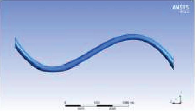
Figure 1 Geometry of the serpentine channel.

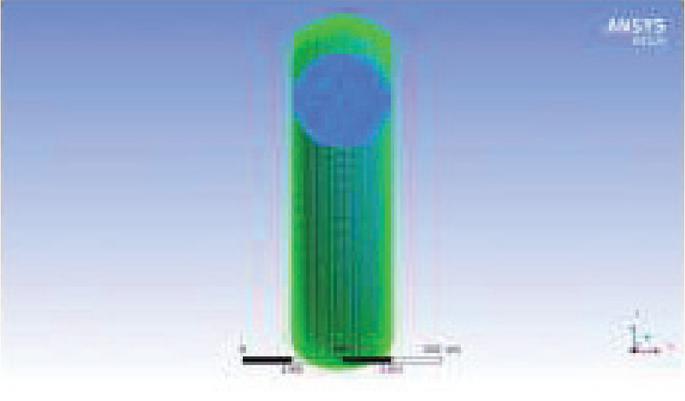
Figure 2 Cross section view of the geometry.

2.1 MESH

Because it is simple to stretch quadrilateral mesh around the corners of the geometry, the computational domain includes quadrilateral mesh on all sides of the geometry. This is because of the ease with which this may be accomplished. A total of about 300 000 000 quadrilateral mesh components are generated for the domain as a whole. An investigation into the sensitivity of the mesh is carried out in order to locate the optimal mesh components, which allows for the achievement of optimal results.

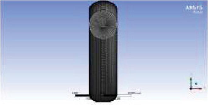
Figure 3 Mesh of the channel.

3 Solution

3.1 Boundary Conditions

The model’s needs should be taken into consideration before applying boundary conditions. At the channel’s intake, [11, 12] a velocity inlet boundary condition with a velocity of 0.50 meters per second is used, and at the outflow, a pressure outlet boundary condition is used. In order to complete the computations, the properties of the Bingham fluid were utilized. The Bingham fluid is investigated using a serpentine channel in both slip and non-slip circumstances. For the purpose of analyzing how fluid behaves inside the channel, several different parameters, such as wall shear stress, turbulent viscosity, static pressure, and others, were investigated in slip and no slip scenarios.

The K-epsilon (k-) turbulence equation was used to tackle the problem that has been bothering us recently. This equation is utilized to investigate the behavior of the Bingham fluid because of its effectiveness in mimicking turbulent flow within the channel. The investigation is being carried out as part of this investigation.

For turbulent kinetic energy (k)

\frac{\partial (ρ k)}{\partial t} + \frac{\partial (ρ k u_{i})}{\partial x_{i}} = \frac{\partial}{\partial x_{i}} [\frac{μ_{t}}{σ_{k}} . \frac{\partial k}{\partial x_{i}}] + 2 μ_{t} E_{i j} E_{i j}

For dissipation ( $ε$ )

\frac{\partial (ρ ε)}{\partial t} + \frac{\partial (ρ ε u_{i})}{\partial x_{i}} = \frac{\partial}{\partial x_{j}} [\frac{μ_{t}}{σ_{ε}} . \frac{\partial ε}{\partial x_{j}}] + C_{1 ε} \frac{ε}{k} 2 μ_{t} E_{i j} E_{i j} - C_{2 ε} ρ \frac{ε}{k}

4 Result and Discussion

4.1 Comparison of Static Pressure for No Slip and Slip Conditions

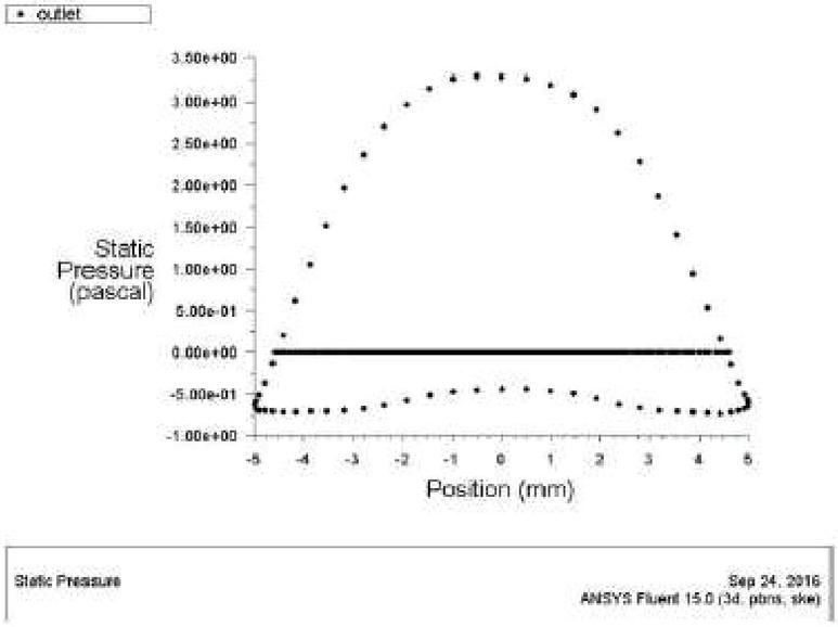
Figure 4 Static pressure in no slip condition.

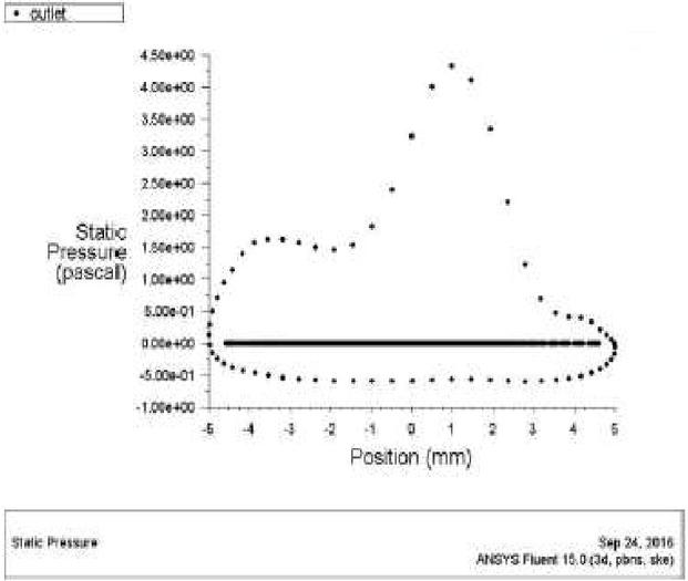
Figure 5 Static pressure in slip condition.

4.2 Comparison of Wall Shear Stress for No Slip and Slip Conditions

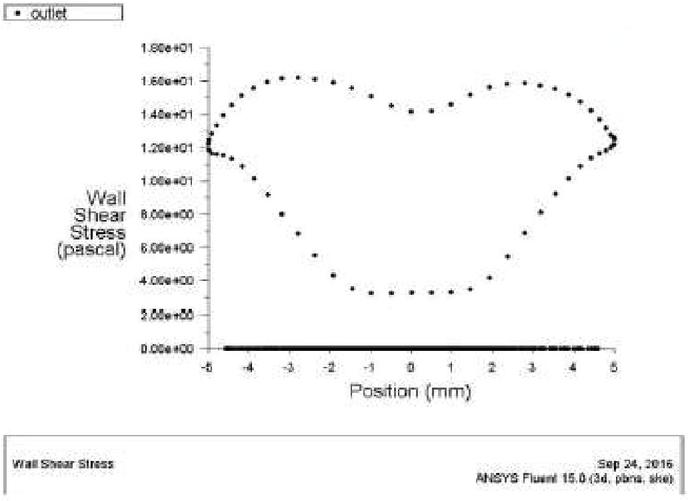
Figure 6 Wall shear stress in no slip condition.

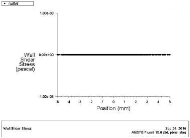
Figure 7 Wall shear stress in slip condition.

4.3 Comparison of Skin Friction Coefficients in Slip and No Slip Conditions

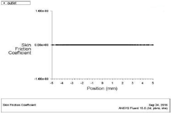
Figure 8 Skin friction co-efficient in no slip condition.

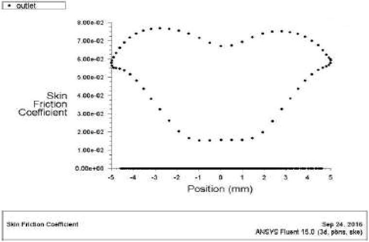
Figure 9 Skin friction co-efficient in slip condition.

It is possible to demonstrate, using the graphs that are shown above, that there is a considerable change in the flow characteristics of Bingham fluid when taking into consideration the fluid in both the slip and no slip circumstances. When there is no slide, the shear forces at the wall are either minimal or linear. This is because fluid does not flow at a constant pace down the whole length of a straight pipe when there is no pulsatile flow. Instead, fluid movement is rapid in the middle but slow around the walls. The velocities of the fluid form a profile that is known as a “laminar flow,” which has the shape of a paraboloid. This kind of flow is created by friction inside the fluid as well as friction between the fluid and the wall of the vessel, and it is affected by the viscosity of the fluid that is being moved. Because of this friction, a tangential force is created by the flowing fluid. This force is known as the “wall shear stress,” and it is caused by the fluid. The rate at which the fluid velocity increased as it went from the vessel wall into the middle of the vessel is the primary factor that establishes the amount of wall shear stress that is present.

The definition of wall shear stress is:

τ_{w} = μ {[\frac{\partial u}{\partial y}]}_{y = 0}

Such variation is also observable in the skin friction coefficients, as is evident from the fact that the local wall shear stress, fluid density, and free-stream velocity are all taken into account when calculating the negligible slip flow of Bingham fluid in serpentine channels. Moreover, such variation is also observable in the skin friction coefficients, as is evident from the fact that such variation is also observable in the skin friction coefficients. The results of this study show that the skin friction coefficients can change in a manner that is analogous to the one described before. In most cases, measurements of these variables are conducted either at the intake or beyond the boundary layer.

5 Conclusion

In the current study, which examines the geology of a serpentine channel for various parameters in slip flow and no slip flow for the same boundary conditions, the Bingham fluid is employed as the working fluid. This fluid is used to assess the geometry of the serpentine channel. It is important to note that the change in parameters for slip and no slip circumstances for the same geometry is quite comparable, and the graphs for the no slip condition are linear. This is something that should be kept in mind. This is something that should be taken into consideration. A Bingham fluid is a type of non-Newtonian fluid that has a yield strength that has to be exceeded before the fluid will flow. This strength must be overcome before the fluid will flow. It is a viscoplastic fluid, which means that when subjected to mild stresses, it behaves like a rigid body, but when subjected to high stresses, it flows like a viscous fluid. Research into curved tubes is absolutely necessary for the efficient operation of businesses that make use of heat exchangers and heat engines.

References

[1] Bigyani Das, Flow of Bingham fluid in a slightly curved tube (1992), International Journal of Engineering Science Vol. 30, No. 9, pp. 1193–1207.

[2] Bayazitoglu, Paslay and Cernocky, Laminar Bingham fluid flow between vertical parallel plates (2007) international journal of thermal science 46 (2007) 349–357.

[3] Fusi and farina, flow of Bingham fluid in non-symmetric inclined channel (2016), journal of Non-Newtonian Fluid Mechanics, JNNFM3783.

[4] Mukherjee, Gupta and Chhabra, Laminar forced convention in power law and Bingham plastic fluids in ducts semi-circular and other cross sections, (2016) International Journal of Heat and Mass Transfer 104 (2017) 112–141.

[5] Shelukhin and Neverov Thermodynamics of micropolar Bingham fluids (2016), journal of non-Newtonian fluid mechanics, JNNFM 3826.

[6] Skelland, Non-Newtonian Flow and Heat Transfer. Wiley, New York (1967).

[7] S. N. BARUA, Q. J. Mech. Appl. Math. 16, 61 (1963).

[8] Kreith, the CRC Handbook of Thermal Engineering, CRC Press, Boca Raton, FL,2000.

[9] Q.M. Lei, A.C. Trupp, Maximum velocity location and pressure drop of fully Develop laminar flow in circular sector ducts, ASME J. Heat Transfer 111 (1989) 1085–1087.

[10] C.Y. Wang, Flow through a lens-shaped duct, ASME J. Appl. Mech. 75 (2008) 034503–034503-4.

[11] Panwar, K, Murthy, D, S, “Analysis of thermal characteristics of the ball packed thermal regenerator”, Procedia Engineering, 127, 1118–1125.

[12] Panwar, K, Murthy, D, S, “Design and evaluation of pebble bed regenerator with small particles” Materials Today, Proceeding, 3(10), 3784–3791.

[13] Bisht, N, Gope, P, C, Panwar, K, “Influence of crack offset distance on the interaction of multiple cracks on the same side in a rectangular plate”, Frattura ed IntegritàStrutturale” 9(32), 1–12.

[14] Panwar, K, Kesarwani, A, “Unsteady CFD Analysis of Regenerator”, International Journal of Scientific & Engineering Research, 7(12), 277–280.

[15] Singh, I., Bajpai, P. K., & Panwar, K. “Advances in Materials Engineering and Manufacturing Processes.