Software Reliability Growth Modeling Based on Fault Count Increment Due to Features Enhancement
Deepti Aggrawal1,*, Adarsh Anand2 and Zuha Shahid2
1USME, East Delhi Campus, DTU, Delhi 42, India
2Department of OR, DU, India
E-mail: deepti.aggrawal@gmail.com; adarsh.anand86@gmail.com; zuhashahid.du.or.21@gmail.com
*Corresponding Author
Received 15 November 2021; Accepted 15 February 2022; Publication 29 March 2022
Abstract
With every up-gradation made in the software there are chances that the number of new faults might creep in the software. This concept has been readily worked upon in the past and is still an active area of research. Software industry has been readily evolving with time and has seen many advancements wherein innovation rate and creation of knowledge has played a pivotal role for continued growth of firms. Often, the use of coming up with new set of features in the base product has brought in answers to many user’s queries. But these up-gradations also known as add-ons also bring in certain new flaws in the software system which is newly created. In the current paper, this fundamental has been worked upon with the help of certain proposed models. Results are supplemented with numerical examples.
Keywords: SRGMs, new feature addition, fault-removal.
1 Introduction
Reliability has always been area of instrumental research and significant improvement in software reliability has demanded new and improvised methods for creating near to perfect software and thereby determining the quality. Software release time is another important and crucial filed wherein; many researchers have immensely contributed. Like the works by eminent scholars; Yamada, Obhaand Osaki [3]; Abdel et al. [4]; Kapur et al. [5], etc. majorly who have contributed in measuring the failure rate of the software. Predicting the field performance has also gained significant attention when it comes to the contributions and literature in this very area (Musa et al. [2]).
Apart from these certain dimensions, people have also studied immensely about the positive aspect of coming up of multi up-gradations in the software system [7–12]. But like it is evident from literature, every side has two coins. There are some bad things associated when you try to dig in some good things. It is this very idea, that we have modelled in this this paper where we have proposed some new mathematical models that talks about the negative impact of coming up of up-gradations after a certain point of time.
In today’s time no product comes with single generation. There are merely any software products available which comes with single generation. Let us take an example of Python Software. Currently the version which is going on is Python 3.10.2, and an important point to note here is that Python 3.9+ cannot be used on Windows 7 or earlier. So, these are certain aspects one has to keep in mind before downloading the software otherwise there are chances that the software might not be installed on the system. One can see the various active versions of the Python Releases in the Table 1 below (https://www.python.org/downloads/):
Table 1 A glimpse of active Python Releases
| Python Version | Maintenance Status | First Released | End of Support |
| 3.10 | bugfix | 4th Oct 2021 | Oct 2026 |
| 3.9 | bugfix | 5th Oct 2020 | Oct 2025 |
| 3.8 | security | 14 Oct 2019 | Oct 2024 |
| 3.7 | security | 27 June 2018 | June 2023 |
| 2.7 | end of life | 3rd July 2010 | January 2020 |
Now as can be seen from the table, the current version is 3.10 and it has very lately been released in the market and the maintenance support will be provided till 2026 and similarly its previous version (Python 3.9) was first release in 2020 and it will be supported till 2025. Like ways the other releases can be understood and it can be observed that each up-grade comes with certain new set of features and enhancements.
Although Goel and Okumoto [1] were the pioneers in the domain of software reliability growth modelling but still they also did not highlight anything with respect to the Software products that comes with multiple versions. Infact, majority of the work proposed in this domain primarily revolved around the thought process revolving around fluctuations in the fault count in its initial count and later count. In other words, they say that the software is understood to go ahead and it penetrates in the “useful life phase” where higher number of flaws gets removed and in accordance, there is a gradual decrement in the failure rate level. One can understand this behaviour with the help of a curve which is given in Figure 1 below.
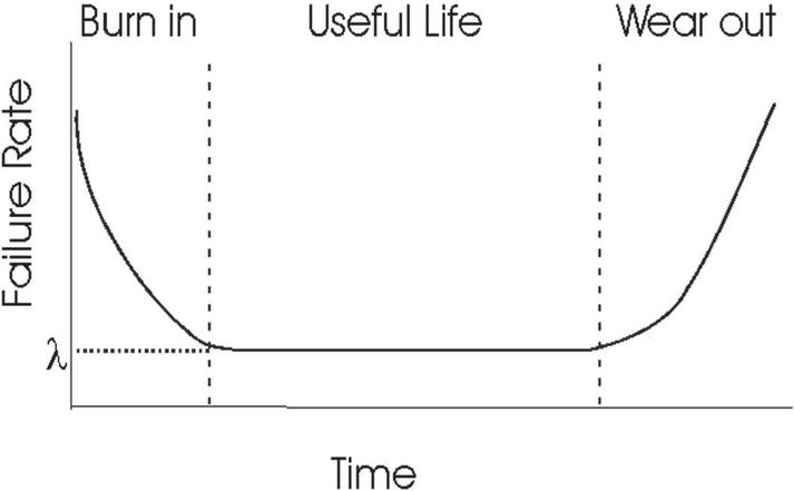
Figure 1 Traditional Failure Curve (Source: Pan [6]).
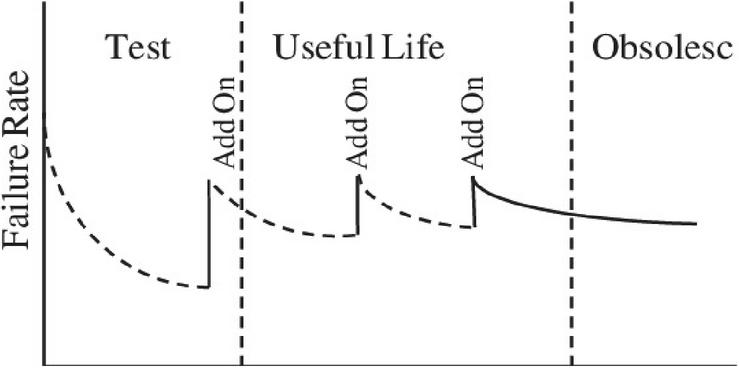
Figure 2 Failure Curve due to Features enhancement (Source: Pan [6]).
It can be observed from the Figure 1 that it is unable to cater to the error growth which might creep in due to the software add-ons or certain new enhancements during the debugging phase. One can look at Figure 2 and understand the behaviour of the failure rate curve. It can be very well seen that during the “useful-life phase”; as any software company undergoes a makeover for the product by features addition or so, the software experiences a radical escalation in failure rate. Now this happens each and every time an upgrade is made in the offering and eventually the failure rate levels off with due course of time. One can associate the finding of the defects and their fixing during this phase to be a reason for the same. Every time any new amendment is done in the software, the complexity is bound to increase and every time we are trying to increase certain functionalities, the chances of more and more errors creeping into the system increases.
As described above, many researchers have extensively worked on this domain, and many studies would be there in the pipeline, but this work discusses the increase in the fault content explicitly after the time point when new additions are being done. Therefore, the objective of this paper is to propose a modelling framework under the assumption that software shall experience a severe intensification in failure count; each time any new feature is added in the product.
Software Reliability Growth Models (SRGMs) have played a significant role in understanding the fault debugging process. A wide variety of models are available in literature for the same. Infect, the domain of multi up gradation has received good attention of the researchers and scholars have extended this concept by inculcating various real life scenarios like those of fault severity, change point, optimal scheduling policy and patching [15–20]. The framework proposed here in this paper is also based on NHPP framework. Using the logistic rate function, the K-G model [13] (which is the building block of this paper) can be understood using the equation given below:
| (1) |
Where denotes the number of faults removed from the software by time . Similarly, , and are usual symbolic representations and their meanings can be understood from the notation section.
The basic assumption of NHPP process can be given as follows.
2 Basic Assumptions
Based on the fundamental of the definition of counting process; and the Non homogeneous Poisson process we also assume that N(t); is a counting process that represents the cumulative fault counts by time t. As described in literature [7–12]; the mean value function (M.V.F) can be shown as below:
| (2) |
And
| (3) |
A model is usually dependent on certain set of assumptions. This proposed framework is also in-line with the assumptions described by [8, 20–22]. But apart from the usual set of assumptions, here we have also considered the fact that fault debugging rate may change at the time point when an up-gradation is done in the software (say after a fix time z).
3 Notations
| a: | Total software defects lying dormant |
| z: | Time after which firms start adding new features. |
| b: | Debugging rate (before time z). |
| b: | Debugging rate (after time z). |
| m(t): | Cumulative number of faults removed. |
| : | Rate of error accumulation (due to feature enhancements). |
| : | Parameter indicating learning behaviour before the time s. |
| : | Parameter indicating learning behaviour after the time s. |
4 Model Development
As described earlier, majority of the work proposed in the domain of error generation has revolved around this increment happening from the beginning. But going by the work done by [21]; wherein they have worked on almost all the types of scenarios and come up with a different articulation altogether, here we have formulated a modeling framework for a software system that incorporates the influence of accumulation of new features in the software. We have tried to mathematically portray the fact that integrating new features might increase software complexity and could result in ending up in having more than usual bugs in the system.
We understand this situation as follows: before any up gradations are made in the software system (that is before time s); the fault content is assumed to remain unchanged. But when new functionalities and new amendments are made in the software code, some new faults creep in the software system. Therefore it is assumed that “the software firm starts incorporating additional features” after time ‘z’ and each extra piece puts in more defects at the rate ‘’. The proposed modeling framework having this dynamicity can be described as follows:
| (4) |
Now, a(t) can take three functional forms as shown in Table 2; and accordingly there will be three different forms of m(t).
Table 2 Different forms of
| Model | I | II | III |
| Before time s | a | a | a |
| After time s |
The following set of differential equations can be framed for the aforesaid proposals and thereby three models can be studied here and solved under the initial set of condition i.e. at
So, For Proposed Model I (PM-I):
| (5) |
And the corresponding mean value function for the aforesaid Equation (5) can be understood as follows:
| (6) |
Similarly, for Proposed Model II (PM-II):
| (7) | ||
| (8) |
For Proposed Model III (PM-III)
| (9) |
Model III is very interesting to note. It talks about addition of faults to the original fault content due to new addendums done in the product. In fact like the other two models, one can see that the parameter (i.e. rate of error accumulation (due to feature enhancements)) plays a noteworthy role all through valuation of the expected number of debugged faults.
5 Data
To illustrate the estimation procedure and application of the proposed SRGMs, validation has been carried out on the real life software failure dataset. This data is taken from Brooks and Motley [14] and comprises of 1301 faults were detected during the testing done for 35 months duration. The size of the radar system software system comprised of 124 KLOC.
6 Parameter Estimation and Comparison
6.1 Model Validation
Model validation is the confirmatory test that is required to check how our model is performing or behaving. In line with this, the parameters of the models under consideration here; are estimated using SPSS Software and the values are given in Table 3.
Table 3 Parameter estimation
| Parameters | PM-I (Equation 6) | PM-II (Equation 8) | PM-III (Equation 10) |
| 1356 | 1322 | 1367 | |
| 0.177 | 0.2133 | 0.222 | |
| 0.226 | 0.2112 | 0.245 | |
| 2.6 | 2 | 3 | |
| 15 | 16 | 18 | |
| 0.064 | 0.063 | 0.059 |
6.2 Model Comparison
The proposed models have been compared with each other on the basis of different comparison criteria like those of; “Mean Square Fitting Error” (MSE), “Coefficient of Multiple Determination” (R) [20, 21], “Bias” [22], “Variation” and last but not the least; “Root Mean Square Prediction Error” (RMSPE) [7–12]. The values are given in Table 4 below.
Table 4 Model comparison
| Parameters | PM-I (Equation 6) | PM-II (Equation 8) | PM-III (Equation 10) |
| 0.994 | 0.998 | 0.997 | |
| bias | 3.071 | 1.833 | 1.166 |
| variation | 69.341 | 76.494 | 51.29 |
| RMSPE | 62.07 | 76.516 | 56.30 |
| MSE | 21523 | 19906 | 12656 |
Now, from Table 3, it is clear that “MSE”, “Bias”, “Variation” and “RMSPE” of the proposed model are nearly equal to each other. The “” value of the proposed model III is moderately greater and for non-beneficial criteria, it is relatively smaller in comparison to that of the other two models. So, Model III performs best for the data set under consideration. Also, the reasonably notable values of makes this assumption more solid and suggests that add-ons in the software plays a vital role in increasing the fault contents. And hence should be taken into account s and when the new advancements are incorporated in the system.
7 Conclusion
The projected models talked about importance of understanding and embedding the feature intensification attribute for studying the reliability growth of the software. The software firms are bound to regularly up-grade themselves and thus, the fault count increment is a natural phenomenon. As and when any new features or add-ons are made in the current offering, software shall experience a drastic proliferation in failure level. Due to the feature up-grades, and addition of new functionalities, the complications in the software as a whole are expected to upsurge. Even when one tries to get hold of these defects some new faults creep in and escalate the total bug count. In this paper, these fundamentals have been worked upon with numerical validation and the results suggest that the rate of error generation due feature enhancements plays a significant role in overall reliability determination of the software.
References
[1] Goel AL, Okumoto K (1979) Time dependent error detection rate model for software reliability and other performance measures. IEEE Transactions on Reliability R-28(3): 206–211.
[2] Musa JD, Iannino A, Okumoto K (1987) Software Reliability: Measurement, Prediction, Application. McGraw- Hill New York, 1:5–15.
[3] Yamada S, Ohba M, Osaki S (1983) S-shaped software reliability growth modelling for software error detection. IEEE Trans on Reliability R-32(5):475–484.
[4] Abdel AA, Chan PY and Littlewood B (1986) Evaluation of Competing Software Reliability Predictions. IEEE Trans on Software Engineering 12 (9):950–967.
[5] Kapur PK, Garg RB, Kumar S (1999) Contributions to hardware and software reliability. Singapore: World Scientific.
[6] Pan J (1999) Software Reliability. Dependable Embedded Systems: 1–15. http://www.ece.cmu.edu/~koopman/des\_s99/sw\_reliability/.
[7] Anand A, Das S, Aggrawal D, Kapur PK (2018) Reliability analysis for upgraded software with updates. In Quality, IT and business operations (pp. 323–333). Springer, Singapore.
[8] Anand A, Gupta P, Tamura Y, Ram M (2020) Software multi up-gradation modeling based on different scenarios. In Advances in Reliability Analysis and its Applications (pp. 293-305). Springer, Cham.
[9] Anand A, Ram M (Eds.) (2020) Systems Performance Modeling (Vol. 4). Walter de Gruyter GmbH & Co KG.
[10] Bhatt N, Anand A, Yadavalli VSS, Kumar V (2017) Modeling and characterizing software vulnerabilities. International Journal of Mathematical, Engineering and Management Sciences: 2(4), 288–299.
[11] Das S, Aggrawal D, Anand A (2019) An alternative approach for reliability growth modeling of a multi-upgraded software system. In Recent advancements in Software Reliability Assurance, pp. 93–105. CRC Press.
[12] Deepika, Singh O, Anand A, Singh JN (2017) Testing domain dependent software reliability growth models. International Journal of Mathematical, Engineering and Management Sciences: 2(3), 40–149.
[13] Kapur PK, Garg RB (1992) A software reliability growth model for an error removal phenomenon. Software Engineering Journal, 7:291–294.
[14] Brooks WD, Motley RW (1980) Analysis of discrete software reliability models – Technical report RADC-TR-80-84. New York: Rome Air development Center.
[15] Singh, O., Anand, A., Aggrawal, D., & Singh, J. (2014). Modeling multi up-gradations of software with fault severity and measuring reliability for each release. International Journal of System Assurance Engineering and Management, 5(2), 195–203.
[16] Singh, O., Aggrawal, D., Anand, A., & Kapur, P. K. (2015). Fault severity based multi-release SRGM with testing resources. International Journal of System Assurance Engineering and Management, 6(1), 36–43.
[17] Deepika, Anand, A., Singh, J., & Singh, J. N. (2019). Modeling change point based multi release software with different fault debugging functions. Nonlinear Studies, 26(3).
[18] Anand, A., Das, S., Agarwal, M., & Yadavalli, V. S. S. (2019). Optimal Scheduling Policy for a Multi-upgraded Software System under Fuzzy Environment. Journal of Mathematical and Fundamental Sciences, 51(3), 278–293.
[19] Das, S., Anand, A., Agarwal, M., & Ram, M. (2020). Release time problem incorporating the effect of imperfect debugging and fault generation: an analysis for multi-upgraded software system. International Journal of Reliability, Quality and Safety Engineering, 27(02), 2040004.
[20] Anand, A., Kaur, J., & Inoue, S. (2020). Reliability modeling of multi-version software system incorporating the impact of infected patching. International Journal of Quality & Reliability Management.
[21] Anand, A., Gupta, P., Tamura, Y., & Ram, M. (2020). Software Multi Up-Gradation Modeling Based on Different Scenarios. In Advances in Reliability Analysis and its Applications (pp. 293–305). Springer, Cham.
Biographies

Deepti Aggrawal is currently working as Assistant Professor at USME, Delhi Technological University, India. She obtained her PhD degree from Department of Operational Research, University of Delhi. She was Operations Manager in Axis Bank till she joined as a research scholar in the Department of Operational Research in 2011. Her Research areas include Marketing and Software Reliability. She is a life member of SREQOM and has publications in journals of national and international repute.

Adarsh Anand did his doctorate in the area of Innovation Diffusion Modeling in Marketing and Software Reliability Assessment. Presently he is working as an Assistant Professor in the Department of Operational Research, University of Delhi (INDIA). He has been conferred with Young Promising Researcher in the field of Technology Management and Software Reliability by Society for Reliability Engineering, Quality and Operations Management (SREQOM) in 2012. He is a lifetime member of the Society for Reliability Engineering, Quality and Operations Management (SREQOM). He is also on the editorial board of International Journal of System Assurance and Engineering management (Springer). He has Guest edited several Special Issues for Journals of international repute. He has edited two books namely: “System Reliability Management (Solutions and Technologies)” and “Recent Advancements in Software Reliability Assurance” under the banner of Taylor and Francis (CRC-Press). He has publications in journals of national and international repute. His research interest includes modeling innovation adoption and successive generations in marketing, software reliability growth modelling and social media analysis.

Zuha Shahid received her B.Sc. in Applied Mathematics from Jamia Millia Islamia, India, in 2019 and M.Sc. in Operational Research from the Department of Operational Research, University of Delhi, India, in 2021. She currently works as a research intern at the Department of Operational Research, University of Delhi. Her current research interest includes software reliability.
Journal of Graphic Era University, Vol. 10_1, 27–40.
doi: 10.13052/jgeu0975-1416.1013
© 2022 River Publishers