Study of the Dependence of Ignition Temperature on the Outer Cone Angle of a Fuel Injector
Subhkaran Singh
Peter the Great Saint Petersburg Polytechnic University, SPBSTU, Department of Atomic and Heat- and -Power Engineering, Saint Petersburg, Russia
E-mail: subhkaran.foam@gmail.com
Received 17 February 2024; Accepted 03 May 2024
Abstract
Internal combustion engines are still a hot topic in research as there is still vast room for improvement. Compression ignition engine research is occurring very rapidly, new diesel blends are being experimented with every day, and duel fuel and tri-fuel diesel engines are becoming a norm. Most of the credit for this research goes to the computation modeling and rapid development of new numerical schemes. This research is one such attempt to capture the spray combustion, using n-heptane as a fuel, with OpenFOAM CFD code. The particles of heptane fuel are injected into the combustion chamber, where the combustion process occurs. The heat transfer between the spray combustion and the surrounding air is realized using the Ranz-Marshall heat transfer model, the mass transfer from the droplets to the surrounding gas due to evaporation and boiling is modeled using the evaporation and boiling model. A conical injector is used for the spray of the fuel and ignition temperature at 20/40/60/ 80/100 thetaOuter is recorded and the results are presented in the form of a graph, showing how 60 is an optimum angle where the ignition temperature is low(not the lowest) and maximum temperature achieved is the highest. This research would be very useful in finding the cone angle of a spray using the various values of thetaOuter, as just by changing the angle of the spray an adverse effect on ignition temperature and maximum temperature is observed. This would allow better ignition temperatures without even changing any other properties of the compression ignition engine. The mesh used is coarse to speed up the calculations, the recorded data shows a change in temperature with various angles, and a bird’s eye view of the flame propagation is also discussed as the change in angle profoundly affects the flame shape.
1 Introduction
Compression ignition engine is the most efficient combustion engine today [1] which is used in the transportation of goods and people on high seas and on the land. The shipping industry relies on diesel engines for its locomotion, even with methanol as a future fuel option, a diesel pilot flame is required for alcohol combustion [9]. Research in internal combustion engines has been going on for a long time, though after the advent of computers and new numerical methods, it has picked up a pace.
This research focuses on the effect of change of the outer cone angle of a fuel injector on the ignition temperature of the fuel (C7H16 in this case) as well as showcases the OpenFOAM’s capability in terms of modeling the combustion process, in a constant volume chamber, filled entirely with air. Many assumptions have been made to simplify the simulation to keep the computational costs low.
2 Combustion
Combustion is an exothermic process that leads to the generation of heat, light in the form of flame and by-products, as it is a chemical reaction between different substances, including oxygen. The reactants combine at a very high rate, firstly because of the nature of the chemical reaction itself and secondly because more energy is generated than can escape to the surroundings, as an outcome the temperature of the reactants is raised even further to accelerate the reaction rate even more so.
2.1 CFD Usage in Combustion
In the understanding of fluid flows to design vehicles, airplanes, etc. no other technique has made such an impact as compared to Computational Fluid Dynamics, which gave rise to digital prototyping. CFD in the past two decades has been extended to combustion-related flows by solving additional conversation equations for individual species [3].
The newly added equations raise a lot of complications on a basic level as they can add up to hundreds of new equations. The tremendous amount of heat released during combustion results in large gradients(spatial and temporal) [3].
The time step required to solve the chemical reactions becomes very small because the source terms of the chemical reactions make the equations very stiff. The conservation equations of reacting flows are similar to those of non- reacting flows, with the exception of the additional species conservation equations for the chemical source terms.
The equation for species conservation: –
| (1) |
where, mass fraction of the species diffusive flux of the species relative to an average mass flux of the fluid is the production of species i, due to chemical reactions
Computation of reacting flows has been used extensively in the past few decades, with various applications from high speed to low speed. The combustion simulation in internal combustion engines is a challenging task as the computational domain keeps changing due to the piston’s movement giving rise to the large volume changes from top to bottom.
2.2 OpenFOAM
Open field operation and manipulation (OpenFOAM) is an open-source C++ library for solving partial differential equations and developing customized solvers, mainly used for computational fluid dynamics created in the 90s by Charlie Hill and Henry Weller. First released in 2004 OpenFOAM has gained a lot of popularity in academia as well as in various industries related to automobiles, manufacturing, chemical firms, etc.
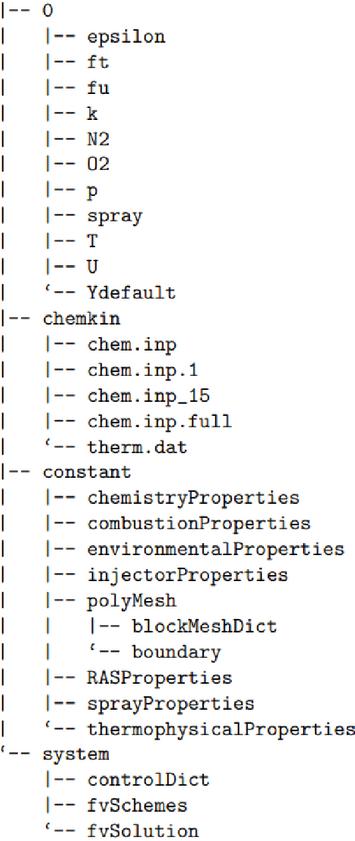
Figure 1 OpenFoam case structure.
OpenFOAM doesn’t have a GUI and runs in the terminal, Figure 1 shows the typical structure of an OpenFOAM case.
3 Geometry
The geometry used in the simulation is a quadrant of a cylinder of the following dimensions and is created in Onshape [4], using data from Table 1, (Figures 1 and 2, show illustrations of the geometry with dimensions):-
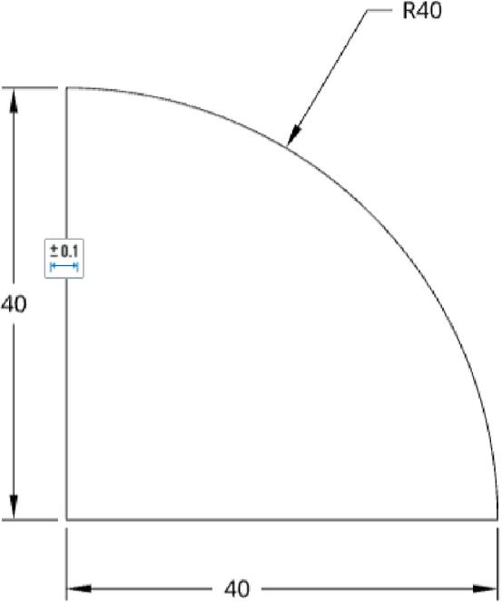
Figure 2 Geometry top view.
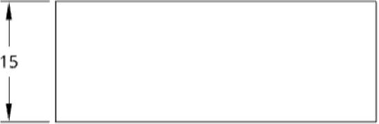
Figure 3 Geometry side view.
4 Meshing
Meshing is done using OpenFOAM’s built-in blockMesh and snappyHexMesh utilities. It uses 38380 cells, and a coarse mesh is used for this simulation to keep the computational costs very low, Figures 3, and 4 show the mesh created.
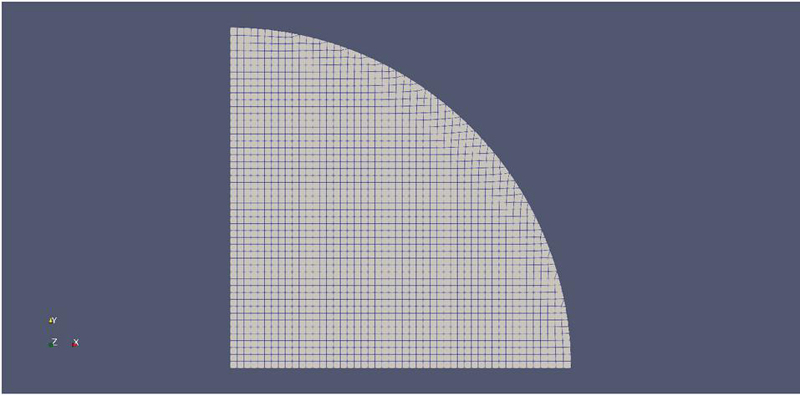
Figure 4 Generated mesh top view.
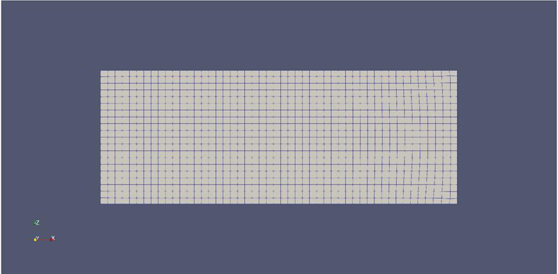
Figure 5 Generated mesh side view.
5 SprayFoam Solver
SprayFoam solver is a transient solver for compressible, turbulent flows with spray particle cloud properties, and is extensively used in spray combustion simulations [4].
6 Combustion Mechanism
ELEMENTS
H O C N AR
END
SPECIES
C7H16 O2 N2 CO2 H2O
END
REACTIONS
C7H16 + 11O2 7CO2 + 8H2O 5.0E8 0.0 15780.0!
FORD/C7H16 0.25/
FORD/O2 1.5/
END
where,
A 5.0E8
b 0.0
Ea 15780.0!
This comes from the Arrhenius rate equation: –
| (2) |
where,
A It is the frequency of correctly oriented collision between the reacting species.
T Temperature
It is the activation energy
forward reaction rate
This Equation (2) determines the rate of chemical reactions as a function of pressure, temperature, and activation energy.
7 Combustion Model
The partially stirred reactor model or PaSR is used in this simulation. This model is widely used in CFD because it allows a very systematic way to account for various chemical and flow time scales. Even though most forms of the implementation of PaSR, represent complex chemical reaction processes with a single time scale.
It assumes that each control volume cell can be divided into two fractions, a reactive (with concentration c) and a non-reactive part. Then due to mixing, interaction occurs between the two fractions with the exchange of mass leading to an outlet concentration C1, as seen in Equation (3).
The reactive part can be shown as: –
| (3) | |
| (4) |
where,
it is the chemical characteristic time
mixing time
when,
| (5) |
It means that mixing is faster than chemistry, and then the model is simplified to the PSR model.
However, it should be mentioned that this model is based on approximations, Equation (4), as there is no actual way to find and .
7.1 OpenFOAM Class of PaSR
| (6) |
where,
it is equal to the Kolmogorov time scale
it is the effective viscosity
it is the turbulent dissipation rate
7.2 Chemical Time Scale
| (7) |
where,
chemical reaction
concentration of total species
number of product species
stoichiometric coefficient
production rate
To calculate the chemical time scale the total species concentration is divided by the rate at which species are transferred from left to right, thus it is computed dynamically based on the chemistry, which makes it very adaptable to the local conditions.
8 Heat Transfer and Phase Change Models
In this research paper, we use the Ranz-Marshall (1952) heat transfer model [8] which takes into account the heat transfer between the spray droplets and the surrounding gas. The evaporation and boiling [9] model is used, to consider the mass transfer from the droplets to the resulting gas due to boiling and evaporation.
| (8) |
where,
Nusselt number
Reynolds number
Prandtl number
heat coefficient
thermal conductivity
these are flow properties determined by the fluid chosen and flow geometry.
9 Discrete Phase Modeling
We input the parameters in the sprayCloudproperties file which contains the sub-models to set up the Lagrangian spray model.
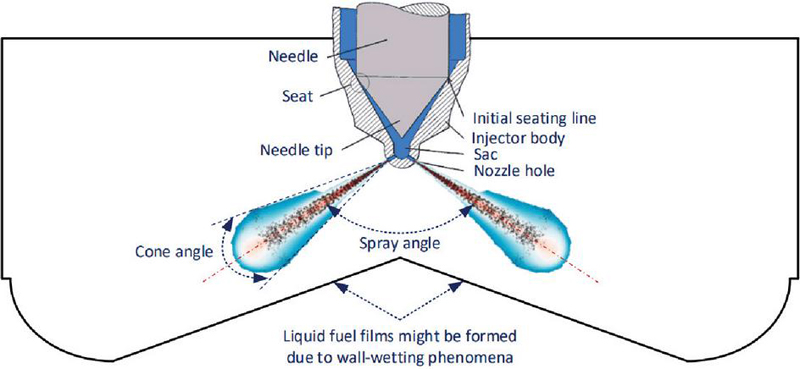
Figure 6 Diagram showing a fuel injector, source [4].
| (9) |
There are 9 injector types available in OpenFOAM, we use the ConeNozzleInjection model as this model is commonly used to deal with conical flow sprays which are frequent in engine combustion simulations.
In this injector model, we input the outer cone angle thetaOuter, Equation (9), (20, 40, 60, 80, 100), which is the agenda of this research.
9.1 The Cone Injector Properties
The purpose of the injector is to introduce the particles in the combustion domain according to the properties of Table 1. The term used for particles used in fluid flow is called a parcel. Parcel is used in simulations and it represents actual real-world particles because to simulate real particles is computationally very demanding. The total mass represents the amount of particle species to be injected in kg. The figure, Figure 6, shows the injector geometry based upon inner and outer cone angles.
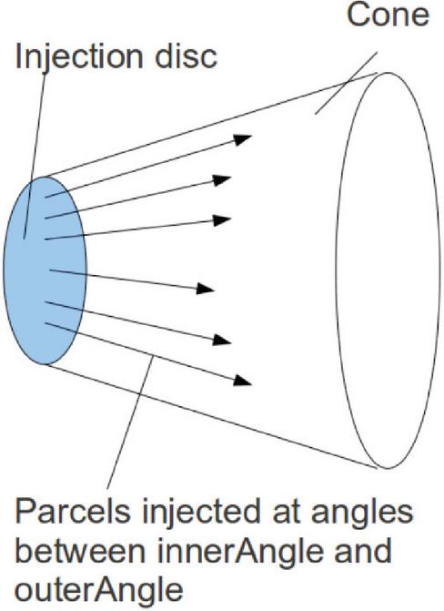
Figure 7 Diagram showing inner and outer cone angles, source [10].
Table 1 Properties of the cone injector
| Total mass[Kg] | 1e-04 |
| Duration[s] | 1e-03 |
| Parcels per second | 10000000 |
| Umg[m/s] | 100 |
| Outer cone angle(thetaOuter) | 20/40/60/ 80/100 |
| Position[x,y,z] | 1e-03, 1e-03, 0.013 |
| Direction[x,y,z] | 1, 1, 0.35 |
9.2 Rosin-Ramler Distribution Model [6]
It is a particle distribution model where random samples are generated from a doubly truncated two-parameter Weibull density function. The random samples are drawn using an inverse transform sampling technique [12].
| (10) |
where,
Rosin-Rammler probability density function
scale parameter
shape parameter
sample
minimum of the distribution
maximum of the distribution
Table 2 Properties of injection distribution
| Min, droplet diameter | 1e-05 |
| Max, droplet diameter | 2e-04 |
| Nominal, droplet diameter | 1e-04 |
| Drag model | Sphere Drag |
| Phase change model | Evaporation and Boiling |
| Turbulence | Realizable K-epsilon |
10 Simulation Parameters
The simulation parameters control the simulation run and in OpenFOAM, reside in the controlDict file in the system folder. The Table 3 shows the main parameters of the controlDict. Application, defines the solver being used, here we are using the sparyFoam solver, then the End Time defines the end of the simulation run and is in seconds. deltaT here is the T of the CFL number,which defines the time step in a transient simulation.
Table 3 controlDict parameters
| Application | sprayFoam |
| End Time | 5e-03 |
| deltaT | 5e-06 |
| maxCo | 0.1 |
11 Results
Figure 8 shows the plot between ignition temperature in Kelvin (y-axis) and time (x-axis), it clearly illustrates the different ignition temperatures for various outer cone angles, also given in tabular form in Table 4. As shown 60 finds a good balance between low ignition temperature and maximum combustion temperature. However, in the future, these results tend to change as more higher fidelity simulations will be performed, with the acquisition of better computational resources.
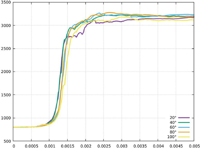
Figure 8 Plot showing the ignition temperature at various angles.
Table 4 Outer cone angle, ignition temperature and time
| Angle | Temperature | Time(s) |
| 20 | 954.587 K | 0.00106374s |
| 40 | 961.485 K | 0.00111670s |
| 60 | 1058.06 K | 0.00123146s |
| 80 | 954.587 K | 0.0010787s |
| 100 | 982.180 K | 0.0018732s |
12 Flame Formation

Figure 9 Flame shape at 20.
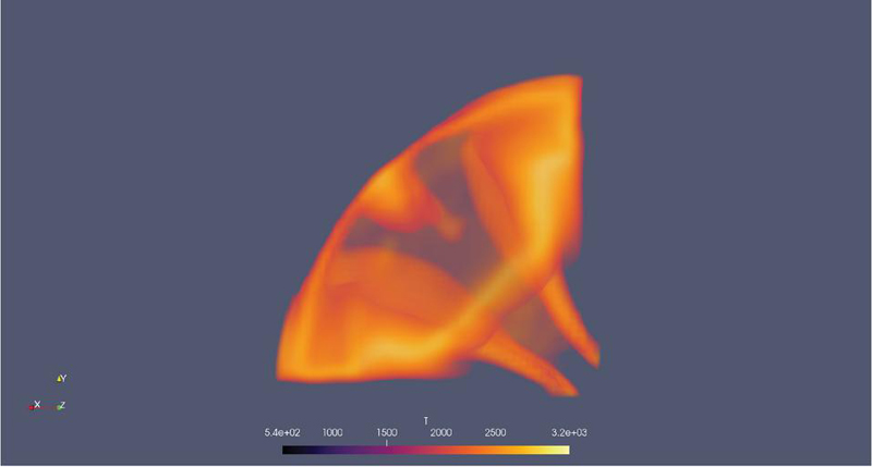
Figure 10 Flame shape at 40.
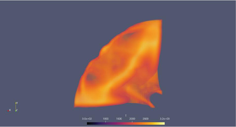
Figure 11 Flame shape at 60.

Figure 12 Flame shape at 80.
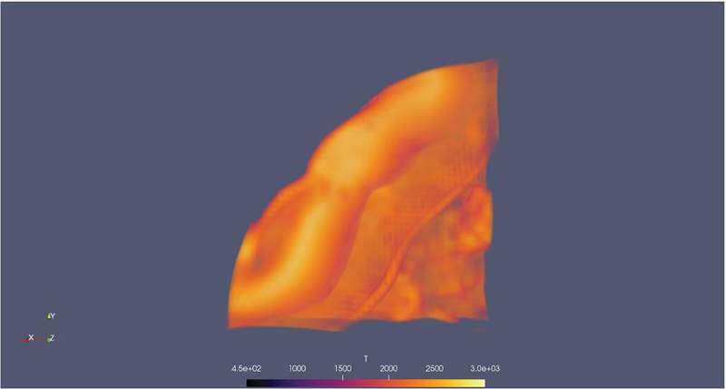
Figure 13 Flame shape at 100.
A change in flame shape is witnessed, as shown from Figures 9 to 13, due to the change in the outer cone angle. The main reason for different flame shapes is attributed to the interaction of spray particles with the walls of the combustion chamber. A thorough insight will be the topic of future research.
13 Conclusion
The study of reliance of ignition temperature on the various angles of the outer cone angle is performed using CFD package OpenFOAM, 20/40/60/ 80/100, outer cone angles are tested. The results show a difference in ignition temperature at different outer cone angles. Suggesting that this method can be used to determine the optimum spray cone angle of compression ignition engines. Further, it is shown that at different cone angles a different flame shape is observed stating the effect on the flame shapes and propagation.
References
[1] Modelling Diesel Combustion 2022 ISBN : 978-981-16-6741-1
[2] The partially stirred reactor model for combustion closure in large eddy simulations: Physical principles, sub- models for the cell reacting fraction, and open challenges.
[3] Duan, Z. et al. Sphere Drag and Heat Transfer. Sci. Rep. 5, 12304; doi: 10.1038/srep12304 (2015).
[4] Pham, V.C.; Le, V.V.; Yeo, S.; Choi, J.-H.; Lee,W.-J. Effects of the Injector Spray Angle on Combustion and Emissions of a 4-Stroke Natural Gas-Diesel DF Marine Engine. Appl. Sci. 2022, 12, 11886. https://doi.org/10.3390/app122311886.
[5] Flow, Turbulence and Combustion https://doi.org/10.1007/s10494-023-00501-7.
[6] Truncated Weibull distribution functions and moments.
[7] Ranz W E and Marshall W R, Jr. Evaporation from drops. Parts I and II. Chem. Eng. Progr. 48:141-6; 173-80, 1952. [University of Wisconsin, Madison, WI].
[8] https://www.openfoam.com/documentation/guides/latest/api/classFoam-1-1combustionModels-1-1PaSR.html.
[9] Yabin Dong, Ossi Kaario, Ghulam Hassan, Olli Ranta, Martti Larmi, Bengt Johansson, High-pressure direct injection of methanol and pilot diesel: A non-premixed dual-fuel engine concept, Fuel, Volume 277, 2020, 117932, ISSN 0016-2361, https://doi.org/10.1016/j.fuel.2020.117932. (https://www.sciencedirect.com/science/article/pii/S0016236120309285)
[10] Description and implementation of particle injection in OpenFOAM.
[11] https://sim-flow.com/.
Biography
Subhkaran Singh is a CFD engineer currently working for an engineering consultancy company in Singapore and at the same time pursuing a PhD in heat transfer. His academic background comprises of Bachelor’s degree in Electrical and Electronics Engineering from Graphic Era University, Dehradun, India, a master’s degree in Power Plant Engineering from Peter The Great Saint Petersburg Polytechnic University, Russia, and another master’s degree in Continuum Mechanics: Fundamental and Applications from the same institute in Russia.
Journal of Graphic Era University, Vol. 12_1, 147–162.
doi: 10.13052/jgeu0975-1416.1219
© 2024 River Publishers