Path Through Specified Nodes and Links in a Network
Santosh Kumar1,* OAM, Elias Munapo2, Philimon Nyamugure3 and Trust Tawanda3
1Department of Mathematical and Geospatial Sciences, School of Sciences, RMIT University, Melbourne, Australia
2School of Economics and Decision Sciences, North West University, Mafikeng Campus, Mafikeng, South Africa
3Department of Statistics and Operations Research, National University of Science and Technology, Box AC 939, Ascot, Bulawayo, Zimbabwe
E-mail: santosh.kumarau@gmail.com; emunao@gmail.com; philimon.nyamugure@nust.ac.zw; trust.tawanda@nust.ac.zw
*Corresponding Author
Received 06 May 2024; Accepted 27 August 2024
Abstract
A constrained shortest route problem in graph theory is about determination of a shortest path between two given nodes of the network that also visits a given set of specified nodes or a set of specified links before arriving to the destination. These earlier approaches did not consider specified elements containing both nodes and links of the given network. This paper finds a shortest path joining the origin node to the destination node, which is constrained to pass through a set of ‘K’ specified elements of the given network, where number of elements represent nodes, , and number of elements represent links, where . Alternatively, if the specified elements representing nodes are contained in the set and the remaining elements representing links by the set , and the set of specified elements denoted by the set then Such restricted path will also have real-life applications. Depending upon the configuration of the specified elements, these constrained paths may have loops. The approach discussed in this paper is a heuristic approach, which finds the required constrained path in a real time.
Keywords: Specified nodes, specified links, specified elements, conditional spanning network, index restricted network.
1 Introduction
Shortest route problem is a classical routing problem which has attracted lot of attention by the researchers, [1–12]. Kalaba [13] modified the shortest route problem by adding a condition that the path joining the origin to the destination must visit a set of specified nodes. Determination of a path through the specified nodes was attempted by the dynamic programming approach by Saksena, Kumar, Sinha and Bajaj [14–16]. The dynamic programming (DP) approach has a disadvantage that its computational complexity increases with an increase in the value of K, and therefore the DP approach had limited success for solving these constrained problems. One more variation of the constrained path problem was proposed and solved by Arora and Kumar, see [17, 18]. The problem they considered was to find the minimum cost route from the origin and the destination, which is constrained to pass through the K specified links of the given network. They solved this problem by using the ring sum linear algebra.
The minimum spanning tree of a given network is also a classical problem in graph theory, which has also been attempted by many, for example, see [9, 19]. The shortest spanning tree problem finds a tree of minimum length of a given network. A variant of the shortest spanning tree was developed by Munapo et al. [20], where the shortest spanning tree was constrained to have restricted node index at node . For example, if the node index at node denoted by , the restriction imposed on the index of the node in [20] is that . This was an interesting variation, which was intended for solving the travelling salesman problem, which requires a minimum cost path that passes through all nodes and returns to the starting node. The index restricted connected network approach was successfully applied by Kumar et al. [21, 22] for solving the travelling salesman problem. Furthermore, this index restricted variation of the minimum spanning tree was also applied by Kumar et al. [23] for solving the constrained path problem posed by Kalaba [13] and observed that computational complexity was no longer dependent on the value K representing the number of specified nodes. Specified node requirement was taken into the account by the index of the node, i.e., and a even number for all specified nodes. Recently Kumar et al. [24] applied the index restricted minimum spanning tree approach [20] to find the constraint path passing through a set of specified links [24].
In this paper, we reconsider the constraint path problem passing through a set of specified elements, where these elements in the set can be:
(i) Nodes only, i.e., when or
(ii) Links only, i.e., when or
(iii) Both, nodes and links, i.e. , where , and .
The (i) above will develop a situation that was discussed by Kumar et al. [23] and the (ii) above will take us to the situation that was discussed by Kumar et al. [24]. In this paper, we discuss the case (iii), that has not been attempted so far. It may be noted that earlier approaches i.e., dynamic programming and liner algebra will not be appropriate when the set , and both sets are not empty, i.e., two sets are such that , and .
A few more relevant algorithms for the shortest route problems can be seen in [25–30].
This paper has been organised in 6 sections. Justification for such a restricted path is discussed in Section 2. Section 3 deals with characteristics of such a path through the K specified elements. Steps of the proposed heuristic for a path through the K specified elements have been discussed in Section 4. A few numerical illustrations are given in Section 5 and concluding remarks in Section 6.
2 Justification for a Path Through K Specified Nodes And links
Distribution and logistics problems arise at every manufacturing site. For a smooth running of the production plant, it is important to make sure that raw materials are made available in time. Manufactured goods must be removed from the production site to warehouses and later forwarded to their destination, the consumer. Many of these distribution and logistics problem are formulated as a network model and solved by using appropriate methodology. Conditions like visiting a set of specified nodes and links in a network model is a natural consequence that may arise in situations, where a scheduled vehicle engaged in doing some tasks is also directed to attend to a specific work at some known places, which can be described by nodes and links of that network.
For example, consider a farm, from where after harvesting, produced must be transported to different warehouses with the intention of raising revenue, retention of produce for personal use, and seeds for the next crop are just a few possibilities. This distribution situations lead to various logistics problems, which can be formulated in the form of a network model. For example, warehouses positions may be represented by the nodes and some outlets on the way from one node to another may be on the links joining those nodes. Such a situation may require finding a path from the origin to the destination, which is constrained to pass through specified elements, which are in the form of nodes and links of the given network.
Another example of a path through nodes and links was recently developed by the strong wind experienced in the city of Melbourne, where lots of trees due to strong winds came down in residential areas and on major highways. These fallen trees got to be removed as a matter of urgency. Councils responsible for these roads must clear the blocked roads as soon as possible. This is a typical situation of looking for a path that must pass through specified links and nodes as these heavy vehicles must enter the road from the correct side to remove the fallen trees.
3 Physical Characteristics of the Constrained Path
Characteristics 3.1: Path May have Loops
We have noted earlier in [23, 24] that a constrained paths may have loops. However, for completeness, let us reconsider a network , where nodes of the network are represented by the set and links are represented by the set , and let cardinality of these two sets be , . It means that the number of nodes and links in the network , is represented by and , respectively. A connected tree of the n node network is comprised of number of links, out of which links have been specified. If the specified links are free of a circuit among them, the additional number of links that will form a connected tree will be . Since specified links are given, they may form any configuration, i.e., a tree, a disconnected graph, or a graph with loops. In addition to specified links, the path to be determined is also required to pass through the specified nodes. Together they all form a part of the path, therefore such a path containing the specified nodes and links may have circuits among them. Since the specified nodes and links are given, they can form any configuration and one such set of specified elements containing nodes and links is shown in Figure 1. Specified elements are shown in blue colour.
As an illustration, in Figure 1 we have two specified links and , and three specified nodes , and , which are displayed in the blue colour. They all must form a part of the path from the origin node 1 to the destination node . This path will pass through the links and , and the nodes , and . In general, we may assume that the number of specified links be denoted by , where is such that and note that inn Figure 1, the value of is equal to 2 and the number of specified nodes is 3.
Since specified links are given, we need at least additional links to form a connected graph of the network , when the specified links did not form any loop, else more links will be required. These additional or more links can be selected by following Kruskal [19] steps, however, such a spanning tree will not be a minimum spanning tree; hence we call it a ‘conditional minimum spanning tree/network’ in [24]. When specified links form a circuit, the network we obtain will not be even a tree and will require links. Additional number of links also reflect the number of circuits in the network. We will again point out this in Section 5.
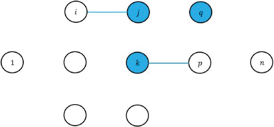
Figure 1 Specified nodes {, and } and specified links {.
Kruskal’s [19] spanning tree approach, can generate a connected graph as explained in the Steps of the algorithm in section 4.
Characteristics 3.2: Nature of the Mathematical model and justification for a heuristic
A mathematical model for this shortest path through K specified nodes and links can be developed but it will be unwieldy and complex for any application, as was explained in [24]. Therefore, a heuristic is desirable for a timely result, which can provide a good solution to the problem in real time.
Characteristics 3.3: Total index, index of specified nodes and nodes associated with specified links.
The number of nodes associated with specified links will be and the number of links in the conditional connected network will be . Therefore, the total index value of all selected and specified links can be .
For specified nodes and nodes associated with the specified links, node index will vary. It may be 2 or 4 for a specified node. For the origin and the destination node, it will be 1, as the path will originate from the origin node and will terminate at the destination node. For a node where a specified link ends or starts, additional link will be required to leave that node or enter that node. Therefore, index for such node will be =2. The path joining the origin to the destination, passing through all specified nodes and nodes associated with the specified links, may require more links for maintaining continuity of the path. This point will be clear in the numerical illustrations. The index value 4 indicates formation of a cycle at that node.
Characteristics 3.4: The ‘Index Balancing theorem’.
The index balancing theorem from [20] states that, a constant when added to all links emanating from the same node does not change the relative merit of any link. However, it can develop an alternative. From the conditional network obtained at Step 1, index values for each node are known, and we also know the desired index values of each node, therefore, the high, and low index nodes can be easily identified. This point is illustrated in the numerical illustrations. Repeated application of the index balancing theorem brings index to a balanced level. Although the index balancing theorem is used to change the links but the specified links cannot be removed by the index balancing theorem. The balancing theorem can be used to increase the index of specified node or a node that belongs to a specified link to an even number.
4 Algorithmic Steps for the Path Through the Specified Nodes and Links
The steps of the algorithm to find the path through the specified nodes and specified links will be as follows:
Step 1: Generate an initial connected network:
1.1 For the given network, select the specified links to form the required initial network. Arrange other links in non-decreasing order of their weight.
1.2. Select the minimum weight link from these links from the step 1.1 and if it forms a cycle with the existing links, reject it. If it does not form a cycle, select it and move to the next minimum weight link. Since the specified links are given, they all are included, even if they may have a cycle among them. However, the subsequent selections should not form a new cycle.
1.3: Repeat Step 1.2, until total number of selected links become . If the specified links form a cycle, for each cycle, additional link will be required to form a conditional connected graph of all n nodes.
Step 2: For the conditional connected network obtained from step 1, develop a table of node index they have, and required for each node. Minimum required index values are estimated by the nature of the node classification. For example, the index value will be at least 2 for a specified node.
Step 3: By the application of the index balancing theorem, bring a balance among the imbalance nodes. When all nodes have attained an index balance, go to Step 4.
Step 4: Find the required path from the origin to the destination, which is passing through the specified nodes and specified links. If path is lacking continuity, go to Step 5.
Step 5: Extra links may be required for developing a path, and they may form a loop. It is illustrated in the numerical illustrations.
5 Illustrative Examples
Two illustrations have been discussed for different configurations of the specified elements.
5.1 Example 1
Consider the network N (10, 21) in Figure 2. Node 1 represents the origin node and destination node is represented by the node 10. The link weights associated with the 21 links are indicated on various links.
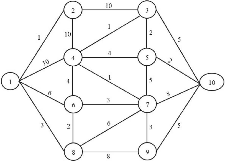
Figure 2 Given network.
The set of specified elements is comprised of nodes and links, where the link set and the node set . This means the set , . Since, both and are not null sets, they form the case (iii) discussed in Section 1, the introduction. Previous approaches dealing with set of specified nodes [23] or the set of specified links [24] will not be applicable to identify the required path. These specified elements are shown in Figure 3. Once again, specified elements are shown in the blue colour.
The minimum node index required by various nods is given in Table 1. Justification for these indices is explained below by an * mark.
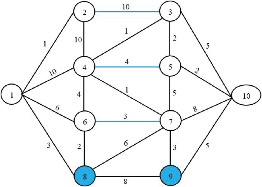
Figure 3 Specified nodes and links of the given network.
Table 1 Node index required
| Node index | 1* | 2** | 3** | 4** | 5** | 6** | 7** | 8*** | 9*** | 10* |
| Required | 1 | 2 | 2 | 2 | 2 | 2 | 2 | 2 | 2 | 1 |
Explanations notes for entries in Table 1:
• *Note that 1 and 10 denote origin and terminal nodes, hence minimum index required is 1 to leave the origin node 1 and to reach the destination node 10.
• ** Nodes 2, 3, 4, 5, 6, 7 from where either a specified link will start or end, which for inclusion in the required path must have one more link to enter or leave that node, hence requirement for the node index will be at least 2 as shown in Table 1.
• *** Since nodes 8 and 9 are specified nodes, index requirement will be at least 2. The total index will be an even number, as when we enter that node, we must leave it also and if we must re-enter it again for some reason, we must leave it again. Total index at such nodes will be an even number and not an odd number.
For the above 10 node networks; the connected network will have 9 links. After selecting the 3 given specified links, we need at least 6 more links to make a conditional connected graph. Since the given specified links are forming a disconnected network; for this configuration, we need to select 6 more links to make a conditional shortest connected network (CSCN). After selecting the 3 specified links, the remaining 18 links are arranged in non-decreasing. Equal weights links are arranged in the order of the first node of that link.
They are given by: {1(1,2) 1(3,4), 1(4,7), 2(3,5), 2(5,10), 2(6,8), 3(1,8), 3(7,9), 4(4,6), 5(3,10), 5(5,7), 5(9,10), 6(1,6), 6(7,8), 8(7,10), 8(8,9), 10(1,4), 10(2,4)}. The specified elements in the form of links are: {10 (2,3), 4(4,5), 3(6,7)}.
Note that the first three links {(1,2), (3,4), (4,7)} are selected for inclusion in the CSCN but the next link (3,5) forms a loop, hence is rejected. Next two links (5,10) and (6,8) are selected for inclusion in the CSCN. Finally, the link (7,9) is selected in the CSCN. This CSCN is shown in Figure 4.
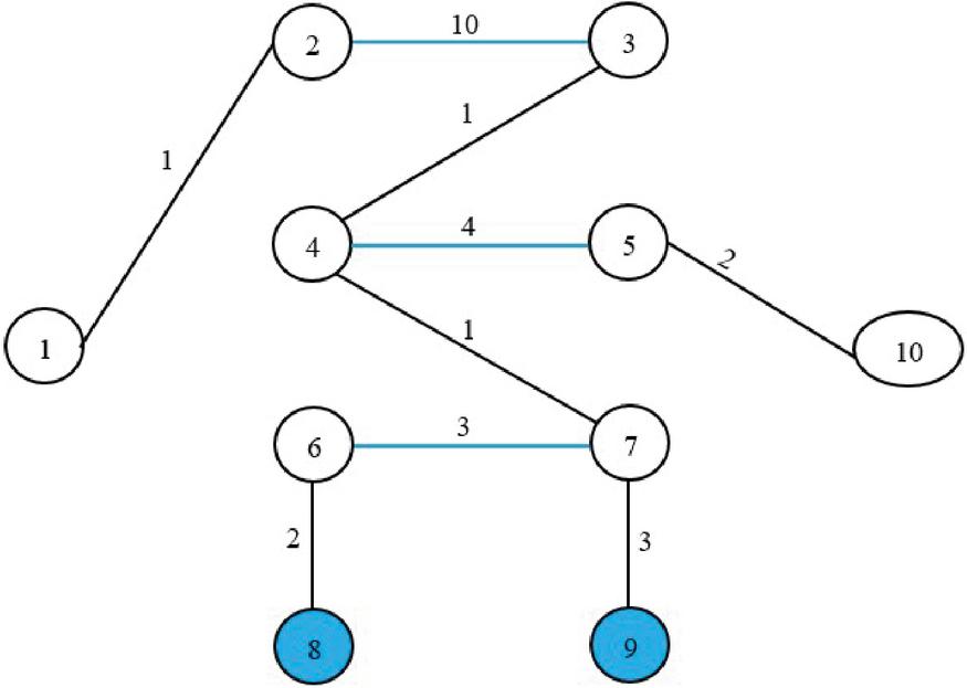
Figure 4 Conditional minimum connected network.
Now we have obtained the CSCN of the given network where all specified elements have been included. Now we plan to compare the node index we have from Figure 4 with the required node index as shown in Table 1. This is shown in Table 2.
Table 2 Node index from Figure 4 is compared with what was required
| Index/ node | 1* | 2** | 3** | 4** | 5** | 6** | 7** | 8 | 9 | 10* |
| Required | 1 | 2 | 2 | 2 | 2 | 2 | 2 | 2 | 2 | 1 |
| Index we have Fig 4 | 1 | 2 | 2 | 3 | 2 | 2 | 3 | 1 | 1 | 1 |
| Imbalance | 0 | 0 | 0 | + 1 | 0 | 0 | +1 | +1 | +1 | 0 |
From Table 2, we note that an imbalance among node index is at node 4, 7, 8, and 9. The imbalance at nodes 8 and 9 can be easily balanced by adding the link (9,8), however, it will give rise to a loop as both nodes are short of one index. This is shown in Figure 5.
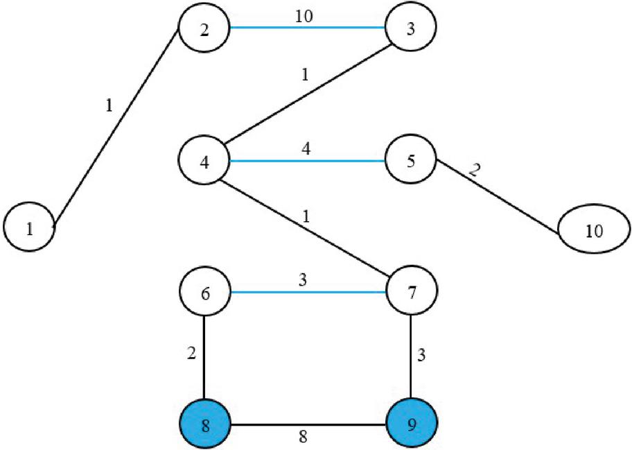
Figure 5 Network after balancing the index of nodes 8 and 9.
The path will be:
1 - 2 - 3 - 4 - 7 - 9 - 8 - 6 - 7 - 4 - 5 - 10.
The above path has 11 links. Since, the connected graph of 10 nodes is expected to have 9 links, if a path pass through all nodes, therefore, the above path will have two circuits, which are:
Circuit 1. 7 - 9 - 8-6 -7,
Circuit 2. 4 -7 - 9 -8 - 6 - 7 - 4,
and note that index at nodes 4 and 7 is not 3 but 4. This is reflected in Figure 6.
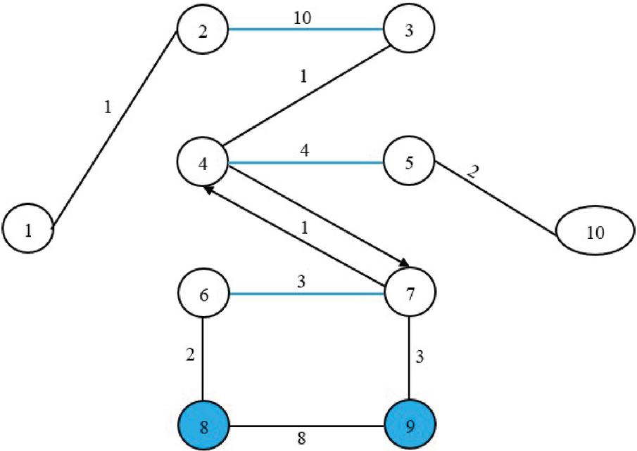
Figure 6 Note the link between the nodes 4 and 7 is acting in both directions like two directed links.
Note from Figure 6, we are having a path from nodes 1 to 10 passing through the specified links {(2,3), (4,5) and (6,7)} and nodes {8, 9}. These new index values are shown in Table 3.
Table 3 Node index values from Figure 4 is compared with what was required
| Index/ node | 1 | 2 | 3 | 4 | 5 | 6 | 7 | 8 | 9 | 10 |
| Required | 1 | 2 | 2 | 2 | 2 | 2 | 2 | 2 | 2 | 1 |
| Index we have | 1 | 2 | 2 | 4 | 2 | 2 | 4 | 2 | 2 | 1 |
| Imbalance | 0 | 0 | 0 | 0 | 0 | 0 | 0 | 0 | 0 | 0 |
The path through the specified links and specified nodes is comprised of two loops, which is typical in a constrained path through specified nodes and links. Once again, note that all node index at the specified nodes and nodes associated with the specified links is effectively an even number as shown in Table 3.
5.2 Example 2
We reconsider the network N(10, 21) in Figure 2 with a slightly different configuration of the specified elements made by links and nodes in Figure 7.
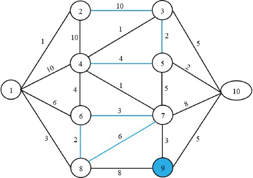
Figure 7 Network with specified elements made of nodes and links.
Note that 6 specified links are: {(2,3), (3,5), (4,5), (6,7), (6,8), (7,8)} and one specified node {9}. To form a CSCN, we need to select at least more links. The remaining non-specified links are 15, which are arranged in non-decreasing order as shown below:
Since the specified links were 6, we need at least 3 more links to form a conditional shortest connected network. These three links are: {(1,2), (4,7), (5,10)}. Note the 3 specified links {(6,7), (6,8) and (7,8)} are forming a loop, and therefore the 9 links will not be able to develop a connected graph. The next link selected is (7,9) forming CSCN with a loop. It is shown in Figure 8, and index is given in Table 4.
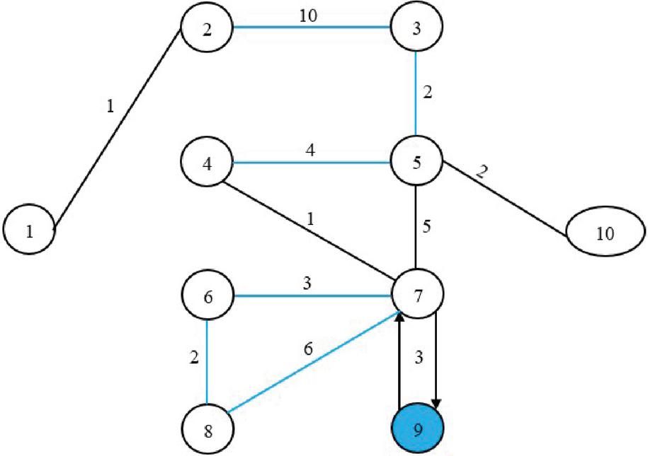
Figure 8 Path through specified nodes and links.
Table 4 Index table for the network in Figure 8
| Index/ node | 1 | 2 | 3 | 4 | 5 | 6 | 7 | 8 | 9 | 10 |
| Required | 1 | 2 | 2 | 2 | 2 | 2 | 2 | 2 | 2 | 1 |
| Index we have | 1 | 2 | 2 | 2 | 4 | 2 | 5 | 2 | 1 | 1 |
| Imbalance | 0 | 0 | 0 | 0 | 0 | 0 | +1 | 0 | +1 | 0 |
Here again the link (7,9) is a two-way link and balance is achieved.
Once all index order is balanced, except the node 9 and node 7, with index value 1 and 5. Since node 9 is a specified node, it can be visited from the link (7,9) and return to node 7. The path is as follows:
, and . Total cost will be =1+10+2+4+1+6+2+3+3+3+5+2 =42 units.
6 Concluding Remarks
6.1 In this paper, we have developed an algorithm to find a route through k specified elements, which can be node and links. Earlier approaches considered specified elements comprised of either node or links but not both.
6.2 Earlier approaches were based on dynamic programming or linear algebra. In dynamic programming, computational complexity was dependent on the value of K and that approach was unable to handle specified links. Similarly, the approach based on linear algebra was able to deal with the specified links only but was unable to deal with the specified nodes. The conditional minimum spanning tree approach used in this paper, can manage K specified elements, where some of these specified elements are nodes and the remaining links.
6.3 Computational complexity does not increase with increase in the number of specified elements which can be in any combination of nodes and links.
6.4 These constrained paths have real-life applications
References
[1] S. Zhang, Z. Luo, L. Yang, F. Teng, and L. Tianrui, A survey of route recommendations: Methods, applications, and opportunities, Information Fusion Volume 108, August 2024, 102413, Elsevier, https:/doi.org/10.1016/j.inffus.2024.102413.
[2] S. Sohrabi, Y. Weng, S. Das, S. Paal, Safe route-finding: A review of literature and future directions, Accident Analysis & Prevention, Vol. 177, 2022, 106816, https:/doi.org/10.1016/j.aap.2022.106816.
[3] H. Joksch, The shortest route problem with constraints, Journal of Mathematical Analysis and Applications, 1966, DOI:10.1016/0022-247X(66)90020-5.
[4] R.K. Ahuja, K. Mehlhorn, J.B. Orlin, and R.E. Tarjan, Faster algorithms for the shortest path problem, Journal of the Association of Computing Machinery, Vol. 37, 1990, pp. 213–223.
[5] R.E. Bellman, Dynamic programming treatment of travelling salesman problems, J of ACM, Vol. 9, 1962, pp. 61–63.
[6] R.E. Beckwith, Dynamic programming and network routing: An introduction to the technique of functional equations, Dynamic programming workshop, Boulder, Colorado, 1961.
[7] G.B. Dantzig, Discrete variable extremum problems, Opns. Res. Vol. 5, pp. 266–76, 1957.
[8] E.J. Dijkstra, A note on two problems in connection with graphs, Numerische Mathematik. 1: 269–271, 1959. doi:10.1007/BF01386390.S2CID123284777.
[9] R.C. Garg, and S. Kumar, Shortest connected graph through dynamic programming, Maths Magazine, Vol. 41, No. 4, pp. 170–73, 1968.
[10] R.M. Peart, R.M. Randolf, and T.E. Bartlet, The shortest route problem, Opns. Res., Vol. 8, pp. 866–868, 1960.
[11] M. Pollack, and W. Weibenson, Solution of the shortest route problem – A review, Opns. Res., Vol. 8, pp. 224–230, 1960.
[12] K. Mehlhorn, P. Sanders, Chapter 10: Shortest Paths, Algorithms and Data Structures: The Basic Toolbox. Springer. Doi:10.1007/978-3-540-77978-0, ISBN 978-3=540-77977-3, 2008.
[13] R. Kalaba, On some communicating network routing problems, Combinatorial Analysis, Proc. Symposium Appl. Math., 10, 1960.
[14] J.P. Saksena, and S. Kumar, The routing problem with ‘K’ specified nodes, Opns. Res., Vol. 14, No. 5, pp. 909–913, 1966.
[15] S.M. Sinha, and C.P. Bajaj, The maximum capacity route through a set of specified nodes, Cahiers du Centre d’Etudes de Recherche Operationnelle, Vol. 11, pp. 133–138, 1969.
[16] S.M. Sinha, and C.P. Bajaj, The maximum capacity route through a set of specified nodes, Opsearch, Vol. 7, pp. 96–114, 1970.
[17] S. Kumar, S., and H. Arora, K shortest paths and paths through R-specified edges in a protean network, ASOR Bulletin, Vol. 14, No. 2, pp. 3–8, 1995.
[18] H. Arora, and S. Kumar, Path through k-specified edges in a liner graph, Opsearch, Vol. 30, No. 2, pp. 163–73, 1993.
[19] J.B. Kruskal, On the shortest spanning tree of a graph and the travelling salesman problem, Proc. Amer. Math. Soc., 7, pp. 48–50, 1956.
[20] E. Munapo, S. Kumar, M. Lesaona, and P. Nyamugure, A minimum spanning tree with node index =2, ASOR Bulletion, Vol. 34, Issue 1, pp. 1–14, 2016. (www.asor.org.au)
[21] S. Kumar, E. Munapo, M. Leasoana, and P. Nyamugure, Is the travelling salesman problem actually NP Hard?, Chapter 3 in Engineering and Technology, Recent Innovations and Research, Editor Ashok Mathani, International Research Publication House, ISBN 798-93-86138-06-4, pp. 37–58, 2016.
[22] S. Kumar, E. Munapo, C. Sigauke, M. Al-Rabeeah, The minimum spanning tree with index =2 is equivalent to the minimum travelling salesman tour, Chapter 8, Mathematics in Engineering Sciences: Novel Theories, Technologies and Applications, ISBN 9781351266321, Editor, Mange Ram, CRC Press (http:/www.crcpress.com) pp. 227–243, 2019.
[23] S. Kumar, E. Munapo, M. Lesaona, and P. Nyamugure, A minimum spanning tree approximation to the routing problem thorough ‘K’ specified nodes, Journal of Economics, Vol. 5, No. 3, pp. 307–312, 2014.
[24] S. Kumar, E. Munapo, P. Nyamugure, T. Tawanda, Minimum spanning tree approach to path through K specified links, Journal of Graphic Era University, Vol. 11, 2, 2023, pp. 221–238.
[25] E. Munapo, B.C. Jones, and S. Kumar, A minimum incoming weight label method and its application to CPM network, ORiON, Vol. 24, South African Journal of OR 2008.
[26] S. Kumar, E. Munapo, O. Ncube, C. Saguke, and P. Nyamugure, A minimum weight labelling method for determination of a shortest route in a non-directed network, Int J Syst. Assur. Eng. Manag. DOI 10.1007/s13198-012-0140-7, Springer, ISSN 0975-6809, Vol. 4, No. 1, pp. 13–18, 2013.
[27] F.B. Zhan, Three fastest shortest path algorithms on real road networks: Data structures and procedures, Journal of the Geographic Information and Decision Analysis, Vol. 1, No. 1, pp. 70–82, 1997.
[28] E. Munapo, and S. Kumar, Linear Integer programming: Theory, Applications, Recent Developments, De Gruyter Publication, ISBN 978-3-11-070292-7, 2022.
[29] C. Zhang, An extended Benders decomposition method for unique shortest path problem, Opsearch, Vol. 61, No. 3, pp. 989–1012, 2024.
[30] S. Kumar, E. Munapo, Innovative ways of developing and using specific purpose alternatives for solving hard combinatorial network routing problems, Applied Math, Vol. 4, pp. 791–805, 2024. https:/doi.org/10.3390/appliedmath4020042.
Biographies

Santosh Kumar OAM received PhD degree in Operations Research from Delhi University. He is author and co-author of over 210 papers and 4 books in the field of Operations Research. His contributions in the field of OR have been recognized in the form of ‘Ren Pots’ award from the Australian Society for operations Research (ASOR) in 2009 and a recognition award from the South African OR Society as a non-member of the society and a non-resident of South Africa in 2011. He was the President of the Asia Pacific Operations Research societies (1995–97), where ASOR was a member along with 7 other countries in the region. He is currently an Honorary Professor at RMIT University, Melbourne. He is a Fellow of the Institute of Mathematics and its Applications, UK. On 14th June 2021, he was awarded a medal of the Order of Australia (OAM).

Elias Munapo holds a BSc. (Hons) Applied Mathematics (1997), MSc. Operations Research (2002) and a PhD Operations Research (2010), all from the National University of science and Technology (N.U.S.T.), Zimbabwe. A certificate in outcomes-based assessment in Higher Education and Open distance learning, University of South Africa (UNISA), certificate in University Education Induction Program, University of KwaZulu-Natal (UKZN). He is a Professional Natural Scientist certified by the South African Council for Natural Scientific Professions (SACNASP), 2012; and NRF rated in South Africa. He has published/co-published over 120 articles and two books. He has also edited/co-edited 7 books and is a guest editor of Applied Sciences, Algorithms and Next Energy journals which are under MDPI. He has supervised/co-supervised eleven doctoral students and over 30 students at Master level. He is a member of the Operations Research Society of South Africa, Executive Committee Member 2012–13, South African Council for Natural Scientific Professions (SACNASP) as a Certified Natural Scientist, European Conference on Operational Research (EURO) and the International Federation of Operations Research Societies (IFORS), and a member of the International Conference on Optimization (ICO) and is part of the team preparing to host ICO 2026 at Johannesburg.

Philimon Nyamugure has a BSc (Hons) 1998, MSc – 2002; Post Graduate Diploma in Higher Education, 2013, all from NUST; PhD in Statistics, University of Limpopo, 2017. He joined NUST in 2003 and was Chairperson for the Departments of Applied Mathematics (2009–2013) and Chairman, Department of Statistics and Operations Research (2013–2019). Became Executive Dean of the Faculty of Applied Science from 2020 to date. A University Senator from 2009 and Councillor from 2020 up to date. He received an award for the best PhD presenter in the School of Mathematical and Computer Sciences, University of Limpopo. Best Senior presenter, Faculty of Applied Sciences, and in 2017 Fulbright Research Award for African Scholars. Involved in several community engagement programs including National University of Science and Technology Schools Enrichment Program (NUSTSEP). He is currently an Executive Dean and a Professor at NUST.

Trust Tawanda is a seasoned academic and researcher with a strong background in Operations Research and Statistics. He holds a Bachelor of Science (Hons) in Operations Research and Statistics (2013), a Master of Science in Operations Research and Statistics (2017), and a PhD in Operations Research (2024) from the National University of Science and Technology (NUST) in Zimbabwe. Currently, he is pursuing a Post Graduate Diploma in Higher and Tertiary Education (PGDHTE) at Great Zimbabwe University (GZU). As a Senior Lecturer in the Department of Statistics and Operations Research at NUST’s Faculty of Applied Sciences, he teaches and conducts research in his areas of expertise, which include network optimization problems, transportation problems, travelling salesman problems, and assignment problems. He has a notable publication record, with papers and book chapters to his credit. His academic journey and research endeavors demonstrate his commitment to advancing knowledge in Operations Research.
Journal of Graphic Era University, Vol. 12_2, 263–282.
doi: 10.13052/jgeu0975-1416.1225
© 2024 River Publishers