Artificial Intelligence (AI) Monitored EOQ Model for Deteriorating Items under Limited Storage Facility, Partial Backlogging and Time Dependent Demand

Sanjay Sharma^*, Anand Tyagi and B. B. Verma

Department of Applied Sciences & Humanities, Ajay Kumar Garg Engineering College, Ghaziabad
E-mail: sharmasanjay@akgec.ac.in; tyagianand@akgec.ac.in; vermabb@akgec.ac.in
*Corresponding Author

Received 29 December 2025; Accepted 30 June 2026

Abstract

In today’s highly competitive markets, the rising cost of warehouse space has become a critical challenge for effective inventory management. This necessitates inventory replenishment policies that explicitly account for limited storage capacity. In this study, we develop an inventory model designed to optimize inventory levels and improve ordering decisions under storage-space constraints. Motivated by the growing influence of Artificial Intelligence (AI) and Machine Learning (ML) in supply chain management implementing AI in this domain requires a structured approach beginning with the collection of high-quality data from diverse sources such as sales records, customer interactions, production logs, and real-time inventory levels. This data must undergo rigorous pre-processing and cleaning to remove inconsistencies and ensure reliability for subsequent analysis. Based on operational needs, suitable AI models – such as machine learning algorithms for demand forecasting, natural language processing for customer inquiries, and computer vision for product identification – can then be selected and trained on historical datasets to identify actionable patterns The data collected support more accurate and timely reorder point decisions. Demand is assumed to be time-dependent, while deterioration is also considered as a time-varying phenomenon. The production rate is finite, shortages are permitted with partial backlogging and the backlogging rate is inversely related to customer waiting time. The objective of the model is to minimize the total inventory cost by jointly determining the optimal cycle length, production rate and order quantity. The effectiveness of the proposed model is demonstrated through a numerical example and a comprehensive sensitivity analysis is conducted to examine the impact of key parameters. The results indicate that incorporating storage constraints and AI-supported reorder decisions can significantly enhance inventory performance and cost efficiency.

Keywords: Artificial intelligence, machine learning, reorder point prediction, inventory control, demand forecasting, time-dependent deterioration, partial backlogging.

1 Introduction

In today’s highly competitive and cost-driven market environment, the efficient utilization of warehouse space has become a critical concern for management across numerous industries. Rising storage costs, expanding product variety, and fluctuating demand patterns compel firms to adopt inventory policies that effectively account for limited storage capacity. When replenishment arrives, excess stock that cannot be accommodated within the available space may result in additional expenses or heightened risk of deterioration – particularly for items with finite shelf lives.

To address these growing challenges, organizations are increasingly turning to Artificial Intelligence (AI) for enhanced order processing. Implementing AI in this domain requires a structured approach beginning with the collection of high-quality data from diverse sources such as sales records, customer interactions, production logs, and real-time inventory levels. This data must undergo rigorous pre-processing and cleaning to remove inconsistencies and ensure reliability for subsequent analysis. Based on operational needs, suitable AI models – such as machine learning algorithms for demand forecasting, natural language processing for customer inquiries, and computer vision for product identification – can then be selected and trained on historical datasets to identify actionable patterns. Fine-tuning model parameters and optimizing algorithms further enhances accuracy and system performance. Once integrated with the existing order management system, these trained models strengthen decision-making functions including order routing, inventory allocation, fraud detection, and customer engagement. Continuous monitoring, feedback collection, and periodic retraining ensure that the AI system remains scalable, adaptive, and aligned with evolving business requirements, while strict adherence to data privacy and security regulations protects sensitive information.

The concept of a two-warehouse inventory system was initially introduced by Hartley [1], who suggested that storing goods in a rented warehouse (RW) generally incurs a higher holding cost than keeping them in an owned warehouse (OW). Building on this foundation, Sarma [2] formulated one of the earliest deterministic models for a deteriorating item with shortages under a constant demand environment using two storage facilities. Later, Pakkala and Achary [3] expanded this framework by allowing a finite production rate and shortages. Subsequent researchers, including Benkherouf [4] and Bhunia and Maiti [5], incorporated time-dependent demand into two-warehouse models for deteriorating products. However, most early studies overlooked the crucial effect of the time value of money, despite the fact that financial performance and investment decisions in real-world businesses are directly linked to inflation and discounting. Recognizing this gap, Buzacott [6] was the first to integrate inflation into inventory modeling and derived a minimum-cost formulation for a single-item system.

Customer willingness to wait for replenishment usually depends on the duration of the waiting period, adding another dynamic factor to inventory decisions. Motivated by these considerations, this paper develops a deterministic inventory model for deteriorating items under storage-space constraints, incorporating time-dependent demand, finite production rate, and partial backlogging. The objective is to minimize total inventory cost by determining the optimal cycle length, production rate, and order quantity. The effectiveness of the proposed model is demonstrated through a numerical example, followed by a comprehensive sensitivity analysis examining the influence of critical parameters such as deterioration rate, inflation rate, and backordering ratio.

2 Literature Review

Beyond technological advancement, practical considerations within inventory systems also necessitate more realistic mathematical models. Many commonly used products – such as perishable foods, pharmaceuticals, radioactive materials, and fragile goods – experience deterioration over time, leading to hidden losses and increased operational costs. Real-world demand further complicates inventory management, as it typically varies with time owing to seasonality, market trends, economic conditions, and promotional activities. Additionally, shortages are often unavoidable, and in many situations allowing shortages with partial backlogging is more economical than holding excessive inventory.

Later, Misra [7] included both internal and external inflation rates along with interest rates, demonstrating their influence on replenishment decisions. Chandra and Bahner [8] extended Misra’s work by considering shortages, while Sarker and Pan [9] studied a finite production rate model with inflation and the time value of money where shortages were allowed. Hariga [10] further advanced this line of inquiry by examining systems with time-dependent demand and shortages in an inflationary context. Bose et al. [11], who formulated an EOQ model for deteriorating items with linear time-varying demand and shortages under inflation and discounting. Van Delft and Vial [12], who adopted a discounted-cost perspective to study items with random and short lifetimes. Moon and Lee [13], who provided a broad review of inflation-affected inventory models. The first attempt to incorporate inflation into a two-warehouse setting was made by Yang [14], who assumed constant deterioration and demand with complete backlogging. Later, Wee et al. [15] introduced partial backordering and Weibull-type deterioration but restricted their study to constant demand and constant backlogging rates. Yang [16] also analyzed partial backlogging in a two-warehouse environment with constant demand under inflation.

Dey et al. [17] developed two-warehouse models incorporating inflation and the time value of money; where Ghosh and Chakrabarty [18] proposed an order-level system with full backlogging. Jaggi and Verma [19] examined a linear trend in demand with complete backlogging under inflation, Patra [20] developed a model with constant deterioration and full backlogging under the time value of money. Two warehouse base inventory control model by Singh et al. [21] developed under partial backlogging for deteriorating items in a two-warehouse structure and Yang [22] later extended earlier models by integrating a three-parameter Weibull deterioration pattern with constant demand.

A closer look at the literature reveals that only a few studies have simultaneously accounted for time-varying deterioration, inflation, and partial backordering, despite these phenomena occurring frequently in real operational environments. The present study addresses this gap by developing a comprehensive inventory model for deteriorating items stored across two warehouses with different deterioration behaviours governed by a two-parameter Weibull distribution. Shortages are permitted and treated as partially backlogged, while demand is assumed to grow exponentially over time. The rented warehouse, as expected, incurs a higher holding cost than the owned warehouse. The model integrates inflation through a discounted cash-flow (DCF) approach and determines the optimal replenishment policy that minimizes the total present value of costs.

Research on EPQ/EOQ models for deteriorating items, two-warehouse systems, and advanced demand structures has grown significantly in recent decades. Early studies explored foundational aspects such as variable holding costs, shortages, and learning effects. For instance, Wang et al. [23] developed deep learning-based demand forecasting in supply chain management and presented a EPQ framework for a two-warehouse system that incorporated variable holding costs and the influence of learning on setup cost, demonstrating how learning can reduce operational expenses over time. In a similar direction, Saha and Chakrabarti [24] investigated deteriorating items with probabilistic demand and variable production rates, contributing to models where uncertainty plays a key role. Further advancements were seen in models addressing delayed deterioration and multi-phase demand patterns. Malumfashi et al. [25] introduced an EPQ model for items with delayed deterioration, incorporating variable production rates and two-phase demand alongside shortages. Dari and Sani [26] extended this idea to situations where demand follows a quadratic pattern, and holding costs are linear, providing a broader understanding of how nonlinear market behavior can influence replenishment decisions.

Multi-warehouse systems have also been central to the literature. Hasan, Kausar, and Verma [27] presented an EOQ model for non-instantaneous deterioration with ramp-type demand within a two-warehouse setting, emphasizing the importance of coordinated warehouse operations. Enhancing this concept, Das [28] incorporated preservation technology and stock-dependent demand into a two-warehouse production model, using a modified genetic algorithm to achieve optimal solutions under complex deterioration behavior. Environmental and green considerations appeared in more recent works. Singh, Singh, and Rani [29] proposed an EPQ model where setup cost depends on population factors in a green environment, highlighting sustainability aspects in production-inventory systems. Likewise, Kumar, Sharma, and Gupta [30] developed a multi-item EOQ model that integrates ramp-type demand, partial backlogging, carbon emission costs, and inflation, showing the increasing importance of environmental and financial factors. Several studies focused on partial backlogging, credit policy, and variable deterioration. Gomathi and Chitra [31] formulated an EPQ model for non-instantaneous deteriorating items with finite production and time-dependent demand, incorporating partial backlogging and credit financing. Kehinde et al. [32] explored EOQ systems for items with delayed deterioration under-price-, stock-, and reliability-dependent demand in a partial backlogging environment. Similarly, Hatibaruah and Saha [33] examined the role of preservation technology investment in systems where demand depends on both time and price.

Models with advanced demand patterns and variable deterioration rates have also been explored. Rabiu and Ali [34] proposed an inventory framework combining linear time-dependent demand, variable holding cost, and backlogged shortages, while Mondal et al. [35] developed an EOQ model with exponential time-dependent demand and backordering. Additional contributions include Padiyar et al. [36], who formulated an EPQ model for two warehouses with different demand and deterioration structures under shortages and imperfect production, and Gupta et al. [37], who introduced an EPQ model incorporating Weibull deterioration and dynamic time-dependent holding costs using Maclaurin series approximations.

Table 1 Comparative analysis of existing literature and the proposed work

				Storage	Finite
	Deteriorating	Time-Dependent	Two-Warehouse	Space	Production	Partial	Inflation/	AI/ML
Reference	Items	Demand	System	Constraint	Rate	Backlogging	TVM	Support
Hartley [1]	$\times$	$\times$	$\mathrm{✓}$	$\times$	$\times$	$\times$	$\times$	$\times$
Sarma [2]	$\mathrm{✓}$	$\times$	$\mathrm{✓}$	$\times$	$\times$	$\mathrm{✓}$	$\times$	$\times$
Pakkala & Achary [3]	$\mathrm{✓}$	$\times$	$\mathrm{✓}$	$\times$	$\mathrm{✓}$	$\mathrm{✓}$	$\times$	$\times$
Benkherouf [4]	$\mathrm{✓}$	$\mathrm{✓}$	$\mathrm{✓}$	$\times$	$\times$	$\times$	$\times$	$\times$
Bhunia & Maiti [5]	$\mathrm{✓}$	$\mathrm{✓}$	$\mathrm{✓}$	$\times$	$\times$	$\times$	$\times$	$\times$
Buzacott [6]	$\times$	$\times$	$\times$	$\times$	$\times$	$\times$	$\mathrm{✓}$	$\times$
Misra [7]	$\times$	$\times$	$\times$	$\times$	$\times$	$\times$	$\mathrm{✓}$	$\times$
Sarker & Pan [9]	$\times$	$\times$	$\times$	$\times$	$\mathrm{✓}$	$\mathrm{✓}$	$\mathrm{✓}$	$\times$
Yang [14]	$\mathrm{✓}$	$\times$	$\mathrm{✓}$	$\times$	$\times$	$\mathrm{✓}$	$\mathrm{✓}$	$\times$
Wee et al. [15]	$\mathrm{✓}$	$\times$	$\mathrm{✓}$	$\times$	$\times$	$\mathrm{✓}$	$\times$	$\times$
Singh et al. [21]	$\mathrm{✓}$	$\times$	$\mathrm{✓}$	$\times$	$\times$	$\mathrm{✓}$	$\times$	$\times$
Mondal et al. [35]	$\times$	$\mathrm{✓}$	$\times$	$\times$	$\times$	$\mathrm{✓}$	$\times$	$\times$
This Work	$\mathrm{✓}$	$\mathrm{✓}$	$\mathrm{✓}$	$\mathrm{✓}$	$\mathrm{✓}$	$\mathrm{✓}$	$\mathrm{✓}$	$\mathrm{✓}$

Recent research also emphasizes multi-stage systems and trapezoidal demand patterns. Suvetha et al. [38] developed a three-stage EPQ model that accounts for time-dependent deterioration and trapezoidal demand dynamics, offering more realistic representations of evolving market conditions. Lastly, Shah, Patel, and Rabari [39] explored inventory decisions under carbon emission constraints, partial backlogging, and price-stock-dependent demand, positioning sustainability at the forefront of inventory management strategies. A numerical illustration and sensitivity analysis highlight the impact of inflation, deterioration rate, and backordering rate on the system’s total cost. The results indicate that relying solely on either rented or owned warehouse storage leads to a higher present-value cost compared to using a coordinated two-warehouse structure.

3 Assumption and notations

3.1 Assumptions

The following assumptions are used in the model;

(i) Reorder point monitoring with AI and ML.

(ii) The retailer continuously observes the inventory status and places an order of size Q whenever the stock level reaches the reorder point R.

(iii) Customer demand occurs in small quantities, so the chance of the inventory dropping below the reorder point due to sudden large withdrawals is negligible.

(iv) The deterioration of items follows a time-dependent pattern.

(v) The demand rate is considered as time dependent.

(vi) The production rate is assumed to be dependent on the prevailing demand rate.

(vii) The retailer has a fixed storage capacity, denoted by W, allocated for stocking the item.

(viii) Any units supplied in excess of the available storage capacity at the time of delivery are sent back to the supplier.

(ix) The retailer’s order quantity is always lower than the available storage capacity.

(x) The duration of shortage (stock-out) within a cycle is relatively small when compared with the total cycle time.

(xi) The supplier imposes an additional charge, calculated as a proportion of the purchasing cost, for each unit returned due to insufficient storage space.

3.2 Notations

Table 2, showing the notations throughout in the model.

Table 2 Notation of the present model

P	=	Production Rate.
T	=	Cycle Time.
$T_1$	=	Duration of production run.
$T_2$	=	Time in which no production but sock is available.
$p_0$	=	Cost of per unit production.
$p_1$	=	Supplier’s per unit selling price.
$p_2$	=	Retailer’s per unit selling price.
$c_{ds}$	=	Cost of per unit deterioration for the supplier.
$c_{dr}$	=	Cost of per unit deterioration for the retailer.
$h_1$	=	Per unit holding cost per unit for the supplier.
$h_2$	=	Per unit holding cost per unit for the retailer.
$\tau$	=	Set up cost for the supplier.
Z	=	The point where reorder initiated for the retailer.
X	=	Lead time demand for the retailer.
W	=	Storage capacity for the retailer.
Q	=	Order quantity for the retailer.
$\eta$	=	Rate of backlogging.
OR	=	Ordering cost for the retailer.
v	=	Stock out time for negative inventory.
Y	=	Demand during lead time for the retailer
T.A.C	=	Total Average Cost

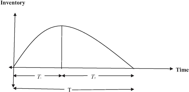
Figure 1 Mathematical representation of the supplier’s model.

4 Model Formulation

4.1 Supplier’s Model

A simple production system is considered, where a single facility manufactures one type of item. The interval between two successive production start points is defined as a cycle. Production begins at the start of each cycle and as items are continuously produced, the inventory rises after satisfying demand and accounting for deterioration. Production continues until time T; after which it stops. Once production halts, the existing inventory depletes due to both demand and deterioration over the remaining part of the cycle. The cycle ends when the inventory level reaches zero. The production begins again at time T.

The differential equations for the system are given by:-

$$\frac{d{I}_s(t)}{dt}+kt{I}_s(t)=(\gamma -1)(a+bt)0\le t\le T_1$$	(1)
$$\frac{d{I}_s(t)}{dt}+kt{I}_s(t)=-(a+bt)T_1\le t\le T_2$$	(2)

With boundary conditions: –

$$I_s(0)=0I_s(T_2)=0$$

(3)

The solution of these equations are given by: –

$I_s(t)$	$=a(\gamma -1)\left(t+{\displaystyle \frac{k{t}^2}{6}}+{\displaystyle \frac{k{t}^3}{6}}\right)e^{-\frac{-k{t}^2}{2}}$
	$+b(\gamma -1)\left({\displaystyle \frac{t^3}{6}}+{\displaystyle \frac{bk{t}^4}{8}}\right)e^{-\frac{k{t}^2}{2}}0\le t\le T_1$	(4)
$I_s(t)$	$=-a\left[at+{\displaystyle \frac{ak{t}^3}{6}}+{\displaystyle \frac{b{t}^2}{2}}+{\displaystyle \frac{bk{t}^4}{8}}\right]e^{-\frac{k{t}^2}{2}}{T}_1\le t\le T_2$	(5)

Now, the total cost for the supplier is given by

${\text{T.C}}_s$	$=\text{Production cost}+\text{deterioration cost}$
	$+\text{inventory holding cost}+\text{set up cost}$	(6)
Production cost	$=p_0{\displaystyle {\int }_0^{T_1}}(\gamma -1)(a+bt)\mathit{d}t=p_0(\gamma -1)\left(a{T}_1+{\displaystyle \frac{b{T}_1^2}{2}}\right)$	(7)

Total deteriorated units $=$ Total production $-$ Total demand

Deterioration cost	$={\mathrm{c}}_{\mathrm{ds}}\left\{(\gamma -1)\left(a{T}_1+{\displaystyle \frac{b{T}_1^2}{2}}\right)-\left(a{T}_2+{\displaystyle \frac{b{T}_2^2}{2}}\right)\right\}$	(8)
Holding cost	$=h_1\left({\displaystyle {\int }_0^{T_1}}{I}_s(t)\right)dt+{\displaystyle {\int }_{T_1}^{T_2}}{I}_s(t))dt$
	$=h_1\{a(\gamma -1)(t+{\displaystyle \frac{k{t}^2}{6}}+{\displaystyle \frac{k{t}^3}{6}})e^{-\frac{-k{t}^2}{2}}$
	$+b(\gamma -1)\left({\displaystyle \frac{t^3}{6}}+{\displaystyle \frac{bk{t}^4}{8}}\right)e^{-\frac{k{t}^2}{2}}$
	$-a[at+{\displaystyle \frac{ak{t}^3}{6}}+{\displaystyle \frac{b{t}^2}{2}}+{\displaystyle \frac{bk{t}^4}{8}}]e^{-\frac{k{t}^2}{2}}\}$	(9)
Set up cost	$=\tau$	(10)

Putting all these values in Equation (6): –

$\text{T.C}(p)$	$=p_0(\gamma -1)\left(a{T}_1+{\displaystyle \frac{b{T}_1^2}{2}}\right)$
	$+{\mathrm{c}}_{\mathrm{ds}}\left\{(\gamma -1)\left(a{T}_1+{\displaystyle \frac{b{T}_1^2}{2}}\right)-\left(a{T}_2+{\displaystyle \frac{b{T}_2^2}{2}}\right)\right\}$
	$+h_1\{a(\gamma -1)(t+{\displaystyle \frac{k{t}^3}{6}}+{\displaystyle \frac{k{t}^3}{6}})e^{-\frac{-k{t}^2}{2}}$
	$+b(\gamma -1)\left({\displaystyle \frac{t^3}{6}}+{\displaystyle \frac{bk{t}^4}{8}}\right)e^{-\frac{k{t}^2}{2}}$
	$-a[at+{\displaystyle \frac{ak{t}^2}{6}}+{\displaystyle \frac{b{t}^2}{2}}+{\displaystyle \frac{bk{t}^4}{8}}]e^{-\frac{k{t}^2}{2}}\}+\tau$	(11)

Total Average Cost (T.A.C(p)) $=$ $\frac{1}{T}{\text{T.C}}_s$

T.A.C(p)

$={\displaystyle \frac{1}{(T_1+T_2)}}{\text{T.C}}_s$

(12)

The total average cost equation can be solving by using optimization method to find the total average cost.

4.2 Buyer’s Model

A buyer-oriented inventory model is formulated under storage-space limitations. When an order of size Q is placed, the quantity that can actually be accommodated in the storage area depends on the inventory level right after the order arrives. Consequently, three distinct scenarios must be considered, based on the relationship among the lead time, the reorder point, the post-delivery inventory level, and the maximum storage capacity (W).

Case 1: – Let us assume that the quantity demanded during the lead time is smaller than the reader point

If Y is the demand during the lead time: –

$\mathrm{R}-\mathrm{Y}\ge 0$ and $\mathrm{R}-\mathrm{Y}+\mathrm{Q}\le \mathrm{W}$

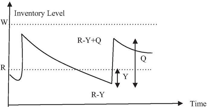
Figure 2 Inventory Level for case-1.

The differential equation governing the transition of the system for the relation is given by: –

$$\frac{d{I}_r(t)}{dt}+Kt{I}_r(t)=-(\gamma -1)(a+bt)0\le t\le T$$
$$I_r(0)=(\mathrm{R}-\mathrm{Y}+\mathrm{Q})$$	(13)

The solution is given by: –

$I_r(t)$	$=\{(R-Y+Q)-a(\gamma -1)(t+{\displaystyle \frac{k{t}^2}{6}}+{\displaystyle \frac{k{t}^3}{6}})e^{-\frac{-k{t}^2}{2}}$
	$+b(\gamma -1)({\displaystyle \frac{t^3}{6}}+{\displaystyle \frac{bk{t}^4}{8}})e^{-\frac{k{t}^2}{2}}\}0\le t\le T$	(14)

The total cost associated with the inventory:

${\text{T.C}}_R$	$=\text{Purchasing cost}+\text{Inv. Holding cost}$
	$+\text{Det. Cost}+\text{Ordering cost}$	(15)
Purchasing cost	$=\mathrm{Q}{p}_1$	(16)
Inv. Holding Cost	$=h_2{\displaystyle {\int }_0^T}{I}_r(t).)dt$
Holding Cost	$=h_2\{(R-Y+Q)T-a(\gamma -1)$
	$\times \left({\displaystyle \frac{T^2}{2}}+{\displaystyle \frac{k{T}^3}{18}}+{\displaystyle \frac{k{T}^4}{24}}\right)e^{-\frac{-k{t}^2}{2}}$
	$+b(\gamma -1)({\displaystyle \frac{T^4}{24}}+{\displaystyle \frac{bk{T}^5}{40}})e^{-\frac{k{t}^2}{2}}\}$	(17)
Total Det. Units	$=\text{Total inventory}-\text{Total demand}$
Total Inventory	$=(R-Y+Q)-a(\gamma -1)\left(t+{\displaystyle \frac{k{t}^3}{6}}+{\displaystyle \frac{k{t}^3}{6}}\right)e^{-\frac{-k{t}^2}{2}}$
	$+b(\gamma -1)\left({\displaystyle \frac{t^3}{6}}+{\displaystyle \frac{bk{t}^4}{8}}\right)e^{-\frac{k{t}^2}{2}}$
Total Demand	$=-{\displaystyle {\int }_0^T}(\gamma -1)(a+bt)\mathit{d}t$
Deterioration Cost	$=\{(R-Y+Q)-(aT+b{\displaystyle \frac{T^2}{2}})C_d$	(18)
Ordering Cost	$=O_R$	(19)

Then Total cost for the retailer in this case: –

$\text{T.C}({\mathrm{R}}_1)$	$=\mathrm{Q}{p}_1+h_2\{({}_2{}^{}\{(R-Y+Q)T+a(\gamma -1)$
	$\times \left({\displaystyle \frac{T^2}{2}}+{\displaystyle \frac{k{T}^3}{18}}+{\displaystyle \frac{k{T}^4}{24}}\right)e^{-\frac{-k{t}^2}{2}}+b(\gamma -1)$
	$\times ({\displaystyle \frac{T^4}{24}}+{\displaystyle \frac{bk{T}^5}{40}})e^{-\frac{k{t}^2}{2}}\})\}+(\mathrm{R}-\mathrm{Y}+\mathrm{Q})$
	$-\left(aT+b{\displaystyle \frac{T^2}{2}}\right)C_d$	(20)
$\text{T.A.C}({\mathrm{R}}_1)$	$={\displaystyle \frac{1}{T}}(T.C{.}_{R1})$	(21)

Case-2: – In this case we have assumed that $\mathrm{R}-\mathrm{Y}+\mathrm{Q}>\mathrm{W}$ This case show that the (R-Y) is non negative. When items received in the inventory then its level exceeds the storage capacity. Then the quantity required that can be accommodated within the available space is (W-(R-Y)). As, inventory is over so retailer has to pay the material return cost for extra inventory as a penalty cost.

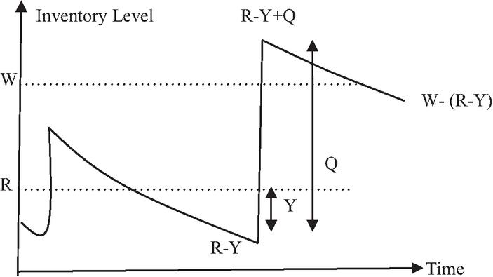
Figure 3 Inventory Level for case-2.

The differential equation governing the transition of the system is given by: –

$$\frac{d{I}_r(t)}{dt}=-kt{I}_r(t)-(\gamma -1)(a+bt)0\le t\le T$$

(22)

With boundary condition: – I${}_r{}^{}(0)=W-(R-Y)$

The solution of this equation is given by: –

$I_r(t)$	$=\{(W-(R-Y))T-a(\gamma -1)(t+{\displaystyle \frac{k{t}^2}{6}}+{\displaystyle \frac{k{t}^3}{6}})e^{-\frac{-k{t}^2}{2}}$
	$+b(\gamma -1)({\displaystyle \frac{t^3}{6}}+{\displaystyle \frac{bk{t}^4}{8}})e^{-\frac{k{t}^2}{2}}\}0\le t\le T$	(23)

Now, the cost for the retailer is given by;

${\text{T.C}}_{R2}$	$=\text{Purchasing cost}+\text{inventory holding cost}$
	$+\text{deterioration cost}+\text{material return cost}$
	$+\text{ordering cost}$
Purchasing cost	$=(\mathrm{W}-(\mathrm{R}-\mathrm{Y}))p_1$	(24)
Holding cost	$=h_2{\displaystyle {\int }_0^T}{I}_r(t)\mathit{d}t$
$H_R$	$=h_2\{(W-(R-Y))T-a(\gamma -1)$
	$\times \left({\displaystyle \frac{T^2}{2}}+{\displaystyle \frac{k{T}^3}{18}}+{\displaystyle \frac{k{T}^4}{24}}\right)e^{-\frac{-k{t}^2}{2}}$
	$+b(\gamma -1)\left({\displaystyle \frac{T^4}{24}}+{\displaystyle \frac{bk{T}^5}{40}}\right)e^{-\frac{k{t}^2}{2}}$	(25)
Deteriorated units	$=\text{Total inventory}-\text{Total demand}$
	$=(W-(R-Y))-{\displaystyle \underset{0}{\overset{T}{\int }}}(\gamma -1)(a+bt)\mathit{d}t$
Deteriorated Cost	$=\{(W-(R-Y))-a(\gamma -1)$
	$\times (t+{\displaystyle \frac{k{t}^2}{6}}+{\displaystyle \frac{k{t}^3}{6}})e^{-\frac{-k{t}^2}{2}}\}c{}_d$	(26)
Ordering Cost	$=O_R$	(27)
Material Returned	$=(\mathrm{R}-\mathrm{Y}+\mathrm{Q}-\mathrm{W})$
Material Returned Cost	$=\alpha p_1(\mathrm{R}-\mathrm{Y}+\mathrm{Q}-\mathrm{W})$	(28)
$\text{T.C}({\mathrm{R}}_2)$	$=(\mathrm{W}-(\mathrm{R}-\mathrm{x}))p_1+\{(W-(R-Y))T$
	$-a(\gamma -1)\left({\displaystyle \frac{T^2}{2}}+{\displaystyle \frac{k{T}^3}{18}}+{\displaystyle \frac{k{T}^4}{24}}\right)e^{-\frac{-k{t}^2}{2}}$
	$+b(\gamma -1)({\displaystyle \frac{T^4}{24}}+{\displaystyle \frac{bk{T}^5}{40}})e^{-\frac{k{t}^2}{2}}\}$
	$\times \{(W-(R-Y))T-a(\gamma -1)$
	$\times \left(t+{\displaystyle \frac{k{t}^2}{6}}+{\displaystyle \frac{k{t}^3}{6}}\right)e^{-\frac{-k{t}^2}{2}}$
	$+b(\gamma -1)({\displaystyle \frac{t^3}{6}}+{\displaystyle \frac{bk{t}^4}{8}})e^{-\frac{k{t}^2}{2}}\}$
	$+\alpha p_1(\mathrm{R}-\mathrm{Y}+\mathrm{Q}-\mathrm{W})+\{(W-(R-Y))$
	$-a(\gamma -1)(t+{\displaystyle \frac{k{t}^2}{6}}+{\displaystyle \frac{k{t}^3}{6}})e^{-\frac{-k{t}^2}{2}}\}c{}_d+O{}_R$	(29)
$\text{T.A.C}(R_2)$	$={\displaystyle \frac{1}{T}}({\text{T.C}}_{R2})$	(30)

Case 3: – When $\mathrm{R}-\mathrm{Y}<0$, it is a shortage of item situation, since the demand during late time is greater than the reorder point.

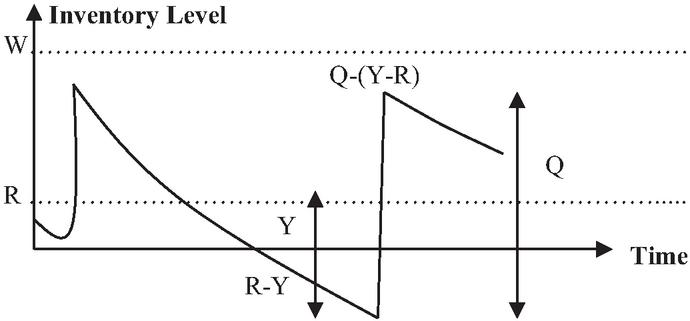
Figure 4 Inventory Level for case-3.

It is assumed that the inventory level starts with shortage at t $=$ 0, it results in shortage. When the stock arrival the maximum inventory level is reaches to $\mathrm{Q}-(\mathrm{Y}-\mathrm{R})$. At $\mathrm{t}=t_v$, after the arrival of stock and satisfying backlogging demand, the inventory level becomes $\mathrm{Q}-(\mathrm{Y}-\mathrm{R})$.

The mathematical equation of the case-3 is as follow: –

${\displaystyle \frac{d{I}_r(t)}{dt}}$	$=-(\gamma -1)(a+bt)0\le t\le t_v$	(31)
${\displaystyle \frac{d{I}_r(t)}{dt}}$	$=-kt{I}_r(t)-(\gamma -1)(a+bt)t_v\le t\le T$	(32)

With boundary conditions: –

$$I_r(0)=0I_r(v)=Q-(Y-R)$$

(33)

The solutions of these equations are given by: –

$I_r(t)$	$=-(\gamma -1)\left(at+{\displaystyle \frac{b{t}^2}{6}}\right)0\le t\le v$	(34)
$I_r(t)$	$=\{Q-(Y-R)T-a(\gamma -1)(t+{\displaystyle \frac{k{t}^2}{6}}+{\displaystyle \frac{k{t}^3}{6}})e^{-\frac{-k{t}^2}{2}}$
	$+b(\gamma -1)({\displaystyle \frac{t^3}{6}}+{\displaystyle \frac{bk{t}^4}{8}})e^{-\frac{k{t}^2}{2}}\}t{}_v\le t\le T$	(35)

Total cost for the retailer in this case is given by: –

$\text{T.C}({\mathrm{R}}_3)$	$=\text{Purchasing cost}+\text{Inv. Holding cost}+\text{Ordering cost}$
	$+\text{Det. Cost}+\text{Shortage Cost}$	(36)
Purchasing cost	$={\mathrm{Qp}}_1$	(37)
Inv. Holding Cost	$=h_2{\displaystyle {\int }_v^T}{I}_r(t)\mathit{d}t$
Holding Cost	$=h_2\{a(vT-{\displaystyle \frac{T^2}{2}})+{\displaystyle \frac{b}{2}}(v^{2}T-{\displaystyle \frac{T^3}{3}})$
	$+{\displaystyle \frac{k}{6}}(v^{3}T-{\displaystyle \frac{T^4}{4}})\}+(Q-(x-R))(1-{\displaystyle \frac{k}{2}}{v}^2)T$
	$-{\displaystyle \frac{ak}{2}}\left({\displaystyle \frac{v{T}^3}{3}}-{\displaystyle \frac{T^4}{4}}\right)-{\displaystyle \frac{k}{6}}{T}^3(Q-(x-R))$
	$-a\left\{({\displaystyle \frac{v^2}{2}}+{\displaystyle \frac{b{v}^3}{3}}+{\displaystyle \frac{k}{8}}{v}^4)\right\}-Q-(x-R))$
	$(1-{\displaystyle \frac{k}{2}}{v}^2)v+{\displaystyle \frac{ak}{24}}{v}^4+{\displaystyle \frac{k}{6}}{v}^3(Q-(x-R))\}$	(38)
Ordering Cost	$=O_R$	(39)
Deteriorated units	$=\text{Total inventory}-\text{Total demand}$
Deteriorated Cost	$=\{(Q-(R-Y))-(\gamma -1)(at+{\displaystyle \frac{b{t}^2}{6}})$
	$-(av+{\displaystyle \frac{b{v}^2}{6}})\}c{}_d$	(40)
Shortage Cost	$=c_s{\displaystyle {\int }_0^v}{I}_r(t)\mathit{d}t$
	$=c_s(\gamma -1)\left(av+{\displaystyle \frac{b{v}^2}{6}}\right)$	(41)
$\text{T.A.C}(R_3)$	$=\{Q-(Y-R)T-a(\gamma -1)(t+{\displaystyle \frac{k{t}^2}{6}}+{\displaystyle \frac{k{t}^3}{6}})e^{-\frac{-k{t}^2}{2}}$
	$+b(\gamma -1)\left({\displaystyle \frac{t^3}{6}}+{\displaystyle \frac{bk{t}^4}{8}}\right)e^{-\frac{k{t}^2}{2}}+Q{p}_1$
	$+h_2\{a(vT-{\displaystyle \frac{T^2}{2}})+{\displaystyle \frac{b}{2}}(v^{2}T-{\displaystyle \frac{T^3}{3}})$
	$+{\displaystyle \frac{k}{6}}(v^{3}T-{\displaystyle \frac{T^4}{4}})\}+(Q-(Y-R))(1-{\displaystyle \frac{k}{2}}{v}^2)T$
	$-{\displaystyle \frac{ak}{2}}\left({\displaystyle \frac{v{T}^3}{3}}-{\displaystyle \frac{T^4}{4}}\right)-{\displaystyle \frac{k}{6}}{T}^3\left(Q-(Y-R)\right)$
	$-a\left\{({\displaystyle \frac{v^2}{2}}+{\displaystyle \frac{b{v}^3}{3}}+{\displaystyle \frac{k}{8}}{v}^4)\right\}-Q-(Y-R))$
	$(1-{\displaystyle \frac{k}{2}}{v}^2)v+{\displaystyle \frac{ak}{24}}{v}^4+{\displaystyle \frac{k}{6}}{v}^3(Q-(Y-R))\}$
	$+O_R+\{(Q-(R-Y))-(\gamma -1)(at+{\displaystyle \frac{b{t}^2}{6}})$
	$-(av+{\displaystyle \frac{b{v}^2}{6}})\}c{}_d+c{}_s(\gamma -1)(av+{\displaystyle \frac{b{v}^2}{6}})$	(42)
	$\text{Total Average Cost}(\text{T.A.C.}({\mathrm{R}}_3))={\displaystyle \frac{1}{T}}\text{T.C}({\mathrm{R}}_3)$	(43)

Now, with the help of the mathematical tolls like Mathematica we can find the optimal solution. In addition, we can use the profit maximization method to find the optimal solution.

5 Numerical Example

To validate the model mathematically, we have taken the following data and calculate the optimal values of $T_1$. The data has been collected from sales records, customer interactions, production logs, and real-time inventory levels.

Inputs: –

$$\mathrm{a}=245,\mathrm{b}=0.3,c_{ds}=10,c_d=21,\gamma =1.5,p_0=7,$$

$$h_1=0.03,h_2=0.04,\mathrm{R}=360,\mathrm{Q}=700$$

$$\mathrm{Y}=260,{\mathrm{T}}_2=18,\mathrm{k}=0.0004,{\mathrm{p}}_1=7.5,\alpha =0.3,$$

$$\mathrm{W}=800,\xi =400,\mathrm{o}=150$$

After solving the optimization equation, the optimal value of $T_1$ found 47. Hence the solution is

Output: –

$$T_1=47$$

6 Sensitivity Analysis

In this section, we have carried out the sensitivity analysis of parameters. The variation in other variable are analysed with respect to the variation in one varilbe.

7 Observations

After studying all the changes in the parameters with respect to the possible changes in the other parameters. The following observations have been seen.

a. The numerical analysis shows that the Total Cost (TAC) attains its minimum value $T_1=47$ & $T_2=18$.

b. From Table 3, it is observed that as the total cycle time $T=(T_1+T_2)$ increases, the time period $T_1$ decreases, while $T_2$ increases. Consequently, the Total Average Cost (T.A.C.) initially decreases.

c. From Table 4, it is observed that when the demand parameter ‘a’ increases, the time period $T_1$ increases, which consequently increases the total cycle time $T=(T_1+T_2)$, while $T_2$ remains fixed at 18. The Total Average Cost (T.A.C.) initially decreases and attains a minimum value at a $=$ 220.

Table 3 Variation in $T_1$ and T.A.C. with the variation in $T_2$

$T_2$	$T_1$	$T_1+T_2$	T.C.	T.A.C.(10-3)
11	41	52	0.185535	3.738
15	42	57	0.102241	2.147
21	31	52	0.238051	4.414
24	28	52	0.350775	6.215
26	26	52	0.509545	9.804
28	23	51	0.494835	9.224
34	13	47	0.231407	5.128
40	5	45	0.83261	19.76

Table 4 Variation in T.A.C. with the variation in demand parameter ‘a’

a	$T_1$	$T_1+T_2$	T.C.	T.A.C.(10-3)
40	–	–	–	–
90	23	41	0.131524	3.5288
130	33	51	–	–
180	39	57	–	–
220	41	59	0.122241	2.14074
370	42	60	0.64841	9.6930
320	44	62	–	–
370	46	64	–	–

Table 5 Variation in T.A.C. with the variation in b

b	$T_1$	$T_1+T_2$	T.C.	T.A.C.(10-3)
$-$1.0	101	119	–	–
$-$1.5	85	103	0.042860	0.42862
$-$2.0	76	94	0.004922	1.05408
$-$2.5	69	87	0.412495	4.91065
0	50	68	0.040951	3.63002
1.0	40	58	0.112241	5.72678
1.5	34	42	–	–
2.0	29	47	–	–
2.5	25	43	0.456480	11.412

Table 6 Variation in T.A.C. with the variation in k

k	$T_1$	$T_1+T_2$	T.C.	T.A.C.(10-3)
.0001	39	57	.194467	2.1234
.00015	40	58	–	–
.0002	40	58	.112241	1.1236
.00025	41	59	–	–
.0003	41	59	.101263	1.6534
.00035	42	60	–	–
.0004	42	60	.158999	2.3678
.00045	43	61	–	–
.0005	44	62	–	–

Table 7 Variation in T.A.C. with the variation in $h_1$ and $h_2$

$h_1$	$T_1$	$T_1+T_2$	T.C.	T.A.C.(10-3)
.03	33	51	.467459	8.7387
.003	36	54	.067074	3.3151
.004	40	58	.112241	2.0407
.005	48	66	.042970	0.7408
.006	–	–	–	–
$h_2$
.04	–	–	–	–
.004	52	70	.476523	7.6532
.050	40	58	.112241	2.0407
.060	34	52	.
.070	31	39	–	–

Table 8 Variation in T.A.C. with the variation in R

R	$T_1$	$T_1+T_2$	T.C.	T.A.C.(10-3)
210	47	65	.529672	8.8122
230	47	65	.402699	6.5036
250	47	65	.375727	4.19503
270	47	65	.212241	3.04074
290	47	65	.148754	.886436
310	47	65	–	–

d. From Table 4, it is observed that when the demand parameter ‘b’ increases, the time period $T_1$ increases, which consequently increases the total cycle time $T=(T_1+T_2)$, while $T_2$ remains fixed at 18. The Total Average Cost (T.A.C.) initially decreases and attains a minimum value at a $=$ 220.

e. It is observed from the Table 5 that as the parameter ‘b’ increases, the time period $T_1$ decreases, which consequently reduces the total cycle time $T=(T_1+T_2)$, while $T_2$ remains fixed. The Total Average Cost (T.A.C.) is minimum at b $=$ $-$1.5. Beyond this value, T.A.C. increases with an increase in ‘b’, indicating that higher values of ‘b’ result in increased operational and holding costs.

f. From Table 6, it is observed that as the deterioration parameter ‘k’ increases, the time period and consequently the total cycle time $T=(T_1+T_2)$, increase, while $T_2$ remains fixed. The Total Average Cost (T.A.C.) initially decreases and attains a minimum value at k $=$ 0.0002.

g. It can be seen from Table 7 that the holding cost parameters $h_1$ and $h_2$ have a significant impact on the replenishment cycle time and the Total Average Cost (T.A.C.). An increase in $h_1$ leads to an increase in the time period $T_1$ and consequently the total cycle time $T=(T_1+T_2)$, while $T_2$ remains fixed. The T.A.C. decreases with an increase in $h_1$.

h. From Table 8, the Total Average Cost (T.A.C.) decreases continuously as R increases and attains its minimum value at R $=$ 290. Beyond this value, feasible solutions do not exist. This indicates that increasing the reorder point reduces the total average cost up to an optimal level.

8 Conclusion

In the current study, an inventory control model for a single item deterministic production inventory model developed. The time dependent rate of deterioration has been assumed and production of the items considered as demand dependent which is a more realistic approaches as per the current market scenario. We have also assumed that the demand to be taken as time dependent and the model being developed in the presence of space restriction. The data which is being collected through sales records, customer interactions, production logs, and real-time inventory levels has been analysed through suitable tools of AI and It has been seen that data collected support more accurate and timely reorder point decisions. Therefore, there is a rich need of AI and its tools for batter analysis of the parameters. It has been also noted that use of AI strongly suggested to monitored the reorder point to avoid unwanted shortage and over inventory both. It is also observed that the reorder point is directly affects the TAC.

9 Future Scope

Although, the current study used all the parameters very carefully and they are designed as per the market trends. But there is always an extension of the available methods. It is suggested to use the other critically designed method of AI like CNN and ML which may be more helpful in the coming time. It is also possible to use Internet of Things (IoT) to enhance supply chain visibility and traceability further. Block chain will be other one potential area of focus.

References

[1] R. V. Hartely, Operations Research – A Managerial Emphasis, Good Year Publishing Company, 1976.

[2] K. V. S. Sarma, “A deterministic order level inventory model for deteriorating items with two storage facilities,” European Journal of Operational Research, vol. 29, no. 1, pp. 70–73, 1987.

[3] T. P. M. Pakkala and K. K. Achary, “A deterministic inventory model for deteriorating items with two warehouses and finite replenishment rate,” European Journal of Operational Research, vol. 57, no. 1, pp. 71–76, 1992.

[4] L. Benkherouf, “A deterministic order level inventory model for deteriorating items with two storage facilities,” International Journal of Production Economics, vol. 48, no. 2, pp. 167–175, 1997.

[5] A. K. Bhunia and M. Maiti, “A two warehouse inventory model for deteriorating items with a linear trend in demand and shortages,” Journal of the Operational Research Society, vol. 49, no. 3, pp. 287–292, 1998.

[6] J. A. Buzacott, “Economic order quantities with inflation,” Operational Research Quarterly, vol. 26, no. 3, pp. 553–558, 1975.

[7] R. B. Misra, “A note on optimal inventory management under inflation,” Naval Research Logistics, vol. 26, no. 1, pp. 161–165, 1979.

[8] M. J. Chandra and M. L. Bahner, “The effects of inflation and the time value of money on some inventory systems,” International Journal of Production Research, vol. 23, no. 4, pp. 723–730, 1985.

[9] B. R. Sarker and H. Pan, “Effects of inflation and the time value of money on order quantity and allowable shortage,” International Journal of Production Economics, vol. 34, no. 1, pp. 65–72, 1994.

[10] M. A. Hariga, “Effects of inflation and time-value of money on an inventory model with time-dependent demand rate and shortages,” European Journal of Operational Research, vol. 81, no. 3, pp. 512–520, 1995.

[11] S. Bose, S. B. Goswami, and K. S. Chaudhuri, “An EOQ model for deteriorating items with linear time-dependent demand rate and shortages under inflation and time discounting,” Journal of the Operational Research Society, vol. 46, no. 6, pp. 771–782, 1995.

[12] C. Van Delft and J. P. Vial, “Discounted costs, obsolescence and planned stock outs with the EOQ formula,” International Journal of Production Economics, vol. 44, no. 3, pp. 255–265, 1996.

[13] I. Moon and S. Lee, “The effects of inflation and time-value of money on an economic order quantity model with a random product life cycle,” European Journal of Operational Research, vol. 125, no. 3, pp. 588–601, 2000.

[14] H.-L. Yang, “Two-warehouse inventory models for deteriorating items with shortages under inflation,” European Journal of Operational Research, vol. 157, no. 2, pp. 344–356, 2004.

[15] H. M. Wee, J. C. P. Yu, and S. T. Law, “Two-warehouse inventory model with partial backordering and Weibull distribution deterioration under inflation,” Journal of the Chinese Institute of Industrial Engineers, vol. 22, no. 6, pp. 451–462, 2005.

[16] H. L. Yang, “Two-warehouse partial backlogging inventory models for deteriorating items under inflation,” International Journal of Production Economics, vol. 103, no. 1, pp. 362–370, 2006.

[17] J. K. Dey, S. K. Mondal, and M. Maiti, “Two storage inventory problem with dynamic demand and interval valued lead-time over finite time horizon under inflation and time-value of money,” European Journal of Operational Research, vol. 185, no. 1, pp. 170–194, 2008.

[18] S. Ghosh and T. Chakrabarty, “An order-level inventory model under two level storage system with time dependent demand,” OPSEARCH, vol. 46, no. 3, pp. 335–344, 2009.

[19] C. K. Jaggi and P. Verma, “Two-warehouse inventory model for deteriorating items with linear trend in demand and shortages under inflationary conditions,” International Journal of Procurement Management, vol. 3, no. 1, pp. 54–71, 2010.

[20] S. K. Patra, “Two-warehouse inventory model for deteriorating items: a study with shortages under inflation and time value of money,” International Journal of Services and Operations Management, vol. 10, no. 3, pp. 316–327, 2011.

[21] S. R. Singh, R. Kumari, and N. Kumar, “A deterministic two warehouse inventory model for deteriorating items with stock-dependent demand and shortages under the conditions of permissible delay,” International Journal of Mathematical Modelling and Numerical Optimisation, vol. 2, no. 4, pp. 357–375, 2011.

[22] H.-L. Yang, “Two-warehouse partial backlogging inventory models with three-parameter Weibull distribution deterioration under inflation,” International Journal of Production Economics, vol. 138, no.1, pp. 107–116, 2012.

[23] Yuan, G., Wu, S., & Wang, B. (2023), “Supply chain management model based on machine learning”, Neural Computing and Applications, 35(6), 4319–4335.

[24] Saha, S., and Chakrabarti, T. (2018), “An EPQ Model for Deteriorating Items with Probabilistic Demand andVariable Production Rate”, American Journal of Engineering Research (AJER), 6, 153–161.

[25] Malumfashi, M. L., Ismail, M. T., Rahman, A., Sani, D., and Ali, M. K. M. (2019), “An EPQ model for delayed deteriorating items with variable production rate, two-phase demand rates and shortages”, International Workshop on Complex Systems Modelling & Simulation (pp. 381–403). Singapore: Springer Singapore.

[26] Sani, Dari, “An EPQ model for delayed deteriorating items with reliability consideration, quadratic demand and shortages”, Pakistan Journal of Statistics and Operation Research (2023): 475–489.

[27] Hasan, A., Kausar, A., and Verma, M. (2021), “An EOQ model for non-instantaneous deteriorating items with ramp-type demand in a two-warehouse facility”, International Journal of Services Operations and Informatics, 11(2–3), 115–158.

[28] Das, D. (2023), “A two-warehouses production inventory model for deteriorating items with stock-dependent demand under preservation technology using modified genetic algorithm”, ICTACT J Soft Comput, 13(4), 3075.

[29] Singh, S. R., Singh, D., and Rani, M. (2023, August), “EPQ model for stock-dependent demand with setup cost dependent on population under green environment, International conference on soft computing for problem-solving (pp. 895–906). Singapore: Springer Nature Singapore.

[30] Gomathi, K., and Chitra, D. (2024), “An EPQ Model For Non-Instantaneous Deteriorating Items With Finite Production Rate And Time Dependent Demand Under The Effect Of Partial Backlogging With Credit Financing Policy”, Frontiers in Health Informatics, 13(5).

[31] Kumar, V., Sharma, A., and Gupta, C. B. (2024), “A multi-item EOQ model for deterioration items with ramp-type demand and partial backlogging under carbon emission and inflationary environment”, International Journal of Operational Research, 51(2), 260–296.

[32] Kehinde, T. O., Shodunke, A. A. A., Bello, K. O., Shoebi, A. O., Aliyu, O. Y., and Abiodun, E. A. (2024), “Economic order quantity (EOQ) for items exhibiting delay in deterioration with price, stock, and reliability demand under partial backlogging”, Science World Journal, 19(4), 1152–1162.

[33] Hatibaruah, A., and Saha, S. (2024), “An inventory system using preservation technology investment for ameliorating and deteriorating items with ramp-type demand dependent on price and time and partial backlogging”, International Journal of Operational Research, 49(4), 431–470.

[34] Rabiu, S., and Ali, M. K. M. (2024), “Optimizing inventory dynamics: a smart approach for non-instantaneous deteriorating items with linear time function dependent variable demands and holding costs, shortages with backlogging”, Journal of Applied Mathematics and Computing, 70(4), 3193–3217.

[35] Mondal, P., Chowdhury, S., Das, P., Majumder, S. K., and De, K. (2024), “An EOQ model for deteriorating item with backorder and time dependent exponential demand”, International Journal of Mathematics in Operational Research, 29(3), 291–308.

[36] Padiyar, S. V. S., Gupta, V., Singh, S. R., and Bhagat, N. (2025), “An EPQ model with different demand and deterioration rate for two warehouses under shortage, learning and imperfect production”, European Journal of Industrial Engineering, 19(2), 109–127.

[37] Gupta, G. K., Nand, A., Chauhan, N. S., and Shivanand. (2025), “An EPQ inventory model with Weibull distribution, dynamic time-dependent holding cost under various demand pattern using Maclaurin series approximations”, Discover Applied Sciences, 7(2), 117.

[38] Suvetha, R., Rangarajan, K., Rajadurai, P., Kaviyarasu, M., and Alqahtani, M. (2025), “Optimized Three-Stage EPQ Model Incorporating Time-Dependent Deterioration and Trapezoidal Demand Dynamics. International Journal of Analysis and Applications, 23, 39–39.

[39] Shah, N. H., Patel, E., and Rabari, K. (2025), “Inventory Decisions with Carbon Emissions, Partial Backlogging and Price-Stock-Dependent Demand”, Sustainable Inventory Management: Perspectives from India (pp. 269–285). Singapore: Springer Nature Singapore.

Journal of Graphic Era University, Vol. 14_2, 407–432
doi: 10.13052/jgeu0975-1416.1424
© 2026 River Publishers