Self-Assembled Peptide Binding to Gold Nanoparticles
Julia Petersen†, Katrine G. Eskildsen† and Peter Fojan*
Department of Materials and Production, Aalborg University, Fibigerstræde 16, 9220 Aalborg Øst, Denmark
E-mail: julia.petersen18@gmx.com; katrine@eskild.cn; fp@mp.aau.com
*Corresponding Author
†These authors have contributed equally to this paper
Received 24 February 2025; Accepted 10 November 2025
Abstract
Self-assembled peptides have been a research focus for the last 50 years. At the same time, metallic nanoparticles have become a subject of interest, especially in the areas of photonics and surface plasmon enhancement. The properties of these two systems, combined with fluorescence, yield a very sensitive bio-assay. To achieve the biosensor, a De Novo peptide has been designed. This novel -helix design contains a recognition motif for a TEV-protease as a model sensor. The prediction of the peptide structure is based on AI-based methods. AlphaFold [1] and PEP-FOLD [2] implementations of the AI algorithms have been used for the analysis. Experimental verification of the peptide properties have been achieved by solid phase peptide synthesis (SPPS) and followed by biophysical methods such as circular dichroism (CD) to verify the secondary structure, atomic force microscopy (AFM) to investigate the self-assembling properties of the gold nanoparticles (AuNPs) and surface plasmon resonance spectroscopy (SPR) for real-time binding and release studies. The experimental data are supplemented with molecular dynamics (MD) simulations. The self-assembly behaviour seen in the MD simulation agrees well with the images obtained by AFM. Simulation of peptide denaturation yields a denaturation temperature above 57∘C.
Keywords: AFM, De novo peptide design, MD simulation, metal nanoparticles peptide biosensor, NAMD simulation, peptide self-assembly.
1 Introduction
Peptides are macromolecules with short chains of amino acids, usually less than 50 amino acids long, and can have various functions, such as anti-bacterial [3], neurotransmitters [4], and toxins [5]. Self-assembling peptides adopt a “bottom-up” strategy, allowing for modifications with both natural and non-natural amino acids within the primary peptide sequence. These can have antimicrobial properties[6] or be peptide hydrogels [7, 8, 9]
Peptides as well as proteins can have various secondary structures such as -helices, -sheets, or random coils. The secondary structure is responsible for the protein and peptide-specific folding architecture [10]. Due to their biophysical similarities, the methods for investigating peptides and proteins are the same.
Protein engineering has for a long time used existing proteins in nature and modified their properties to adjust or alter their functions. With the advent of improved AI methods, the De Novo protein design is able to probe a larger folding space than hitherto accessible. The self-assembly of -helical and coiled coil peptides has a long history in protein and peptide design [8, 10, 11].
During the last decades, computational methods have become faster and more accurate in predicting protein structures [12]. For the De Novo design [13] of peptide and protein structures [14] PEP-FOLD [2] as well as AlphaFold [1] have been applied. PEP-FOLD [2] is optimised to predict secondary structures of peptides, based on Hidden Markov Models [15]. Predictions with AlphaFold [1] are done nowadays by AI techniques, based on multiple sequence alignments (MSA) [16].
In 1977 the first molecular dynamics simulation was made for a folded protein. Nowadays, MD simulations are applied to provide insight into the natural dynamics of biomolecules in solutions. It is also used to simulate thermal averages of molecular properties and to determine at which conformation a molecule or complex is thermally stable [17].
Nanoparticles can exist in various forms, but some are particulate dispersions of solid particles. They are often in the size range of 10–1000 nm. In the 1960s Professor Peter Paul Speiser from ETH in Zürich created a nanoparticle with the purpose of drug delivery and for vaccines. Different geometries, such as spherical, cylindrical and triangular, can be formed depending on the applied method [18, 19].
AuNPs have been used for centuries to stain glass windows to obtain a vibrant ruby colour. Faraday has already described the synthesis of colloid AuNPs and studied their interaction with light. Apart from gold, he also experimented with other materials such as zinc, iron, and stannum. In the last decade, metal nanoparticles have become the center of research again and can be found nowadays in more than 1000 products. AuNPs for example are applied in drug delivery, the detection of genetic-diseases and disorders, tumor detection, photothermal therapy, and high-resolution imaging [20, 21]
Metal nanoparticles can be produced with either a “bottom-up” or “top-down” approach, in contrast to self-assembling peptides which can only be produced with “bottom-up”. For peptides, it would be the fmoc SPPS [22].
The peptide has been designed to self-assemble and bind to AuNP, via the sulfur atom of cysteine at the C-terminus of the -helix. At the N-terminus a fluorophore (5(6)-carboxyfluorescein) has been incorporated. To ensure stable incorporation of AuNP into the peptide -helix, two cysteines at the C-terminus have been added, see Figure 1. The AuNPs used for the experiments have been produced according to the method proposed by Suchomel et al. (2018) [23].
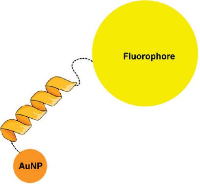
Figure 1 Schematic model of the binding of the peptide and AuNP. The binding between the AuNP and the peptide is obtained through two cysteine residues. The fluorophore is located at the N-terminus.
2 Method
2.1 SPPS
SPPS has been performed on an Activo-P11 peptide synthesiser (Version 1.4.4.32). The temperature has been set to 50∘C throughout the synthesis. Fmoc-Rink-Amid-MBHA resin with a loading capacity of 0.550 mmol/g has been used for the synthesis. The primary solvent for the synthesis was Dimethylformamide (DMF), the activator used was HBTU/Oxyma Pure, and N,N-Diisopropylethylamin (DIEA) served as a base. Piperidine has been used to deprotect after each coupling cycle. Finally, the peptide has been washed in Dimethyl carbonate (DCM) in order to remove remaining DMF. The peptide has been cleaved from the resin on a Activo-P12 cleavage station.
The cleavage mix was as follows:
• 92.5 Trifluoroacetic acid (TFA)
• 2.5 Triisopropylsilane (TIS)
• 2.5 1,2-Ethanedithiol (EDT)
• 2.5 Dionised (DI) water
After 40 minutes of cleavage, the reactor was emptied and washed with 4 mL of TFA.
2.2 Synthesis of AuNPs
For the synthesis of AuNPs, a solution consisting of 25 mmol/L Tween80 and 5 mmol/L tetrachloroauric acid was continuously stirred at room temperature, while adding DI-water to obtain a volume of 15 mL. Subsequently, 20 mL of 25 mmol/L glucose and 25 mmol/L sodium hydroxide solution were added. After 30 minutes, the solution changes color from slight yellow to purple, indicating the completion of the reaction [23].
2.3 Mixture of Peptide and AuNPs
The cleaved peptides were dissolved in 0.1% TFA/milli-Q water by an ultrasonic bath, and the AuNPs were dissolved in milli-Q by use of a vortex. The mixture of dissolved peptide and AuNPs were then combined by the use of a vortex. The concentration of AuNPs in the stock solution was 1 mmol/L, which was mixed with either the 10 M or 86 M peptide solution, giving a 1:10 ratio AuNPs to peptide solution. No further purification steps were executed before further analysis.
2.4 CD
In order to verify the designed peptide structure, a CD spectrum has been recorded on a Jasco J-715 CD spectropolarimeter with a Peltier temperature-controlled cell, between 190 nm and 300 nm. For the thermal denaturation curve, the CD signal was followed at 222 nm. The denaturation curve is measured between 20∘C to 85∘C, with a scan speed of 90 .
Under the assumption of a two-state unfolding model of the peptide, the midpoint of unfolding () together with thermodynamic parameters can be extracted from the change in ellipticity, , with temperature according to Equation (2.4). [24]
| (1) |
where is the midpoint of the transition, is the unfolding enthalpy, is the specific heat capacity of the unfolding, is the gas constant and , , and are the standpoint and slopes of the native and denatured region, respectively. is the ellipticity at 298 K and is the extrapolated ellipticity at 298 K. and are the slopes that account for the linear dependencies of the ellipticities with temperature in the native and denatured regions.
2.5 AFM
AFM images are recorded at random locations on an NT-MDT Ntegra in air. All the samples have been analysed with a tip from NuNano, SCOUT 150 RAI. The parameters of the tip can be seen in the Table 1. All the images were line scans made by tapping mode. The AFM images have been analysed with WSxM [25].
Table 1 Cantilever information used for the NT-MDT Ntegra
| Spring | Resonant | Tip |
| Constant | Frequency [] | Radius [] |
| 18 | 150 | 10 |
2.5.1 Deposition on wafer
To deposit solutions on the surface of the silica wafer, a positive charge is needed. 750 L Toulene and 250 L APTES were mixed. The mixture and the clean wafers were placed in a desiccator. After evacuation of the desiccator for 15 minutes, the wafers and the silanisation mixture were left to react for one hour. 20 L of the solution were deposited onto freshly silanised wafers and left for 30 minutes, rinsed with DI-water and carefully dried under a stream of nitrogen. This was done for both the AuNPs and the mixture of peptide and AuNPs. The same procedure is performed to deposit solutions to the surface of the mica wafer with the exception of the silanisation process.
2.6 Surface Plasmon Resonance
SPR measurements were performed on a dual-channel Reichert2SPR. The temperature is kept constant at 25∘C with milli-Q water as a running buffer. Binding curves were recorded with a flow rate of 20 L/min.
2.7 Fluorescence Spectroscopy
Fluorescence spectroscopy was performed on an ISS Chronos DFD spectrophotometer. Liquid samples were loaded into a quartz cuvette with a path length of 1 cm. All spectra were recorded in the wavelength range between 500 nm and 600 nm.
2.8 MD Simulation
The self-assembly process of the peptide is investigated with the help of MD simulations. Coarse-grained simulations are perfomed with GROningen Machine for Chemical Simulations (GROMACS) [26] to analyse the self-assembly of the peptide. AlphaFold [1] and PEP-FOLD [2] were used to predict the atomic coordinates of SSGQFYLNE(AL)2(AQ)3AGCC of the peptide. In order to simulate thermal denaturation, the Nanoscale Molecular Dynamics (NAMD) [27] has been used.
Snapshots of coarse-grained MD simulations and thermal denaturation simulations were captured using Visual Molecular Dynamics (VMD) [28]. Changes in structure during the different simulations are quantified using the Solvent Accessible Surface Area (SASA) calculated by GROMACS [26]. Summary of the software, used to perform MD simulations is shown in Table 2.
Table 2 Software used to perform MD simulations
| Software | Version |
| Ubuntu | 20.04 |
| AlphaFold | 1.5.2 |
| PEP-FOLD | 3.5 |
| martinize.py | 2.6.3 |
| martini forcefield | v2.2 |
| Gromacs | 2022.4 |
| NAMD | 2.14 |
| Python | 3.8.10 |
| VMD | 1.9.3 |
3 Results and Discussion
3.1 Rational Sensor Design
The designed -helix structure of the peptide consists of a combination of hydrophobic- and hydrophilic amino acids, alanine (A) and glutamine (Q) respectively. These amino acids are known to give a strong -helix structure and avoid steric hindrance problems. The -helix structure does not originate in nature, making it a de novo design. Figure 2(a) shows the -helix with both recognition sites for the TEV protease and the two cysteines. It can be seen that the entire sequence provides a good prediction of the peptide structure, with plDDT values above 80 and above 90 for the core helical structure. The TEV recognition site is located at the N-terminus end of the peptide.
The structure of the peptide has been predicted with AlphaFold [1] and PEP-FOLD [2], see Figure 2. It could be seen that the PEP-FOLD [2] predicted structure, see Figure 2(b) is different from the AlphaFold [1] prediction, see Figure 2(a). PEP-FOLD [2] predictions result in a shorter -helix structure, leaving the TEV recognition site in a random coil conformation.
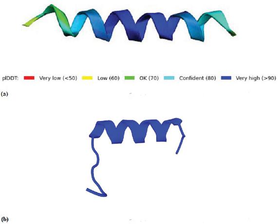
Figure 2 (a) The structure prediction of peptide in AlphaFold [1]. (b) The structure prediction of in PEP-FOLD [2].
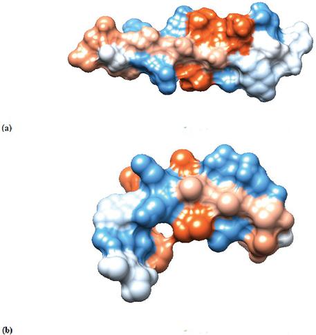
Figure 3 (a) The Van der Waals surface of predicted by AlphaFold [1]. (b) The Van der Waals surface of predicted by PEP-FOLD [2].
The Van der Waals surface (Figure 3) of the predicted structures shows the hydrophobic and hydrophilic parts of the peptide. The blue and red areas indicate the hydrophilic and hydrophobic areas of the peptide, respectively. The prediction from AlphaFold [1] shows a more planar peptide, see Figure 3(a). Whereas the PEP-FOLD [2] structure predicts a curved peptide, and thereby explains the differences in surface areas, see Figure 3(b).
4 Experimental Verification of Design Criteria
The peptide is produced by fmoc SPPS and is expected to have a crude yield of 93. However, HPLC measurements show a pure yield of 46, equivalent to 289 mg. This low yield compared to the theoretical yield can be explained by the coupling reactions during peptide synthesis. Several factors can affect the yield, such as steric hindrance and/or racemization.
The CD spectrum of the designed peptide dissolved in TFA/milli-Q water, see Figure 4(a), shows two minima in the range of [200–240] nm, indicative for an -helix. The temperature scan of the peptide followed by CD at 220 nm was fitted to Equation (2.4), see Figure 4(b). Thermodynamical parameters obtained from the fitting are summarised in Table 3. The peptide is stable up to 37∘C where the onset of melting starts and is completely denatured at 57∘C. The melting temperature of the peptide is around 45∘C.
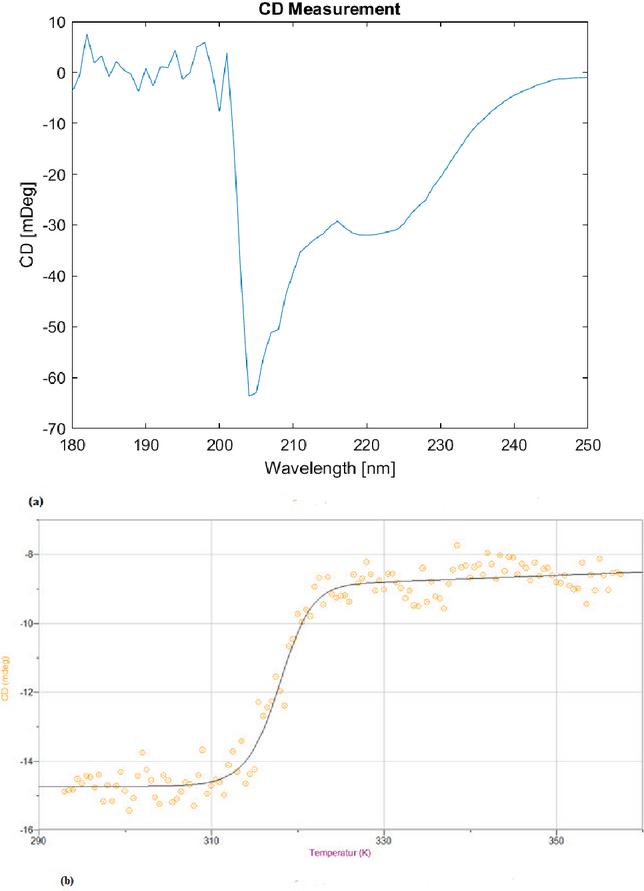
Figure 4 (a) CD spectrum recorded on the spectropolarimeter. (b) CD thermal denaturation curve measured at 222 nm of 5(6)-Carboxyfluorescien-SSGQFYLNE(AL)2(AQ)3AGCC and approximated with Equation (2.4).
Table 3 , H and S obtained from approximation of CD temperature scan with Equation (2.4)
| 317.8 K | |
| H | |
| S | |
| RMSE | 0.419 |
The denaturation of the peptide can also be seen in the simulation performed with Namd, where the peptide denatures over time as a result of high temperatures. For determination of the conditions for the thermal stability of the peptide, one peptide is placed in a box with water. The last frame where the peptide is stable is at 146 ns, see Figure 5(a). After 150 ns, the peptide is completely unfolded into a linear peptide, see Figure 5(b), and subsequently reorders itself into a random coil, see Figure 5(c).
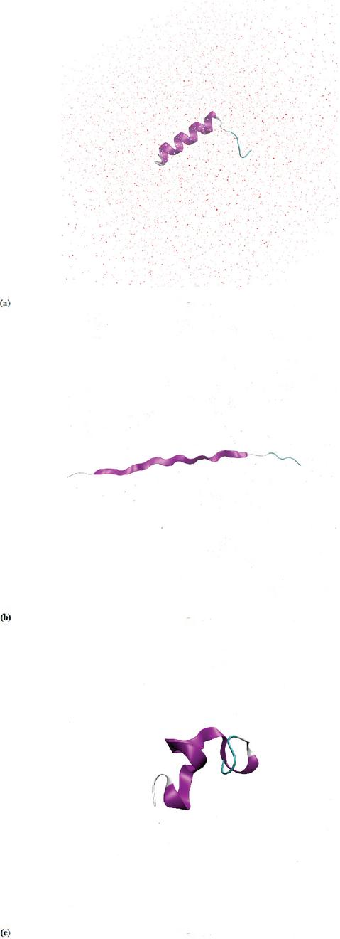
Figure 5 NAMD simulation of thermal stability of the peptide. The blue, purple and white represent the peptide and the red particles represent the water molecules. (a) The beginning of the simulation at 144 ns. (b) The middle point of denaturation at 146 ns. (c) The end of simulation at 150 ns.
To investigate the binding properties of the peptide to Au, a bare flat Au surface in an SPR has been used. A SPR sensogram of the dissolved peptide solution in 0.1% TFA/mili-Q water binding is shown in Figure 6. In the figure, the red line indicates the beginning of peptide injection onto the Au surface. After 3.6 minutes, the flow is stopped and the peptide on the surface is left to bind to the surface. This can be seen in the sensogram as the signal rises additionally from 300 RIU to 450 RIU. After 10.6 minutes, the Au surface was washed with milli-Q water (blue line). The orange line in the sensogram corresponds to the time in which the non specific bound peptide has been removed from the Au surface.
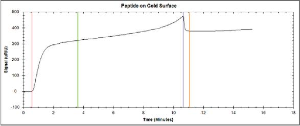
Figure 6 SPR sensogram shows the binding of the dissolved peptide solution in 0.1% TFA/mili-Q water to a clean gold surface. The red vertical line indicates the injection of 10 M peptide. The green line indicates the end of injection of the peptide. Blue line indicates start of washing with milli-Q water. Orange line indicates the end of washing with milli-Q water.
The emission spectrum of the peptide bound to AuNPs in an aqueous solution shows a broad maximum at around 525 nm, see Figure 7. This corresponds to the maximum emission of carboxyfluorescein, indicating that the flurophore has been successfully conjugated with the peptide [29].
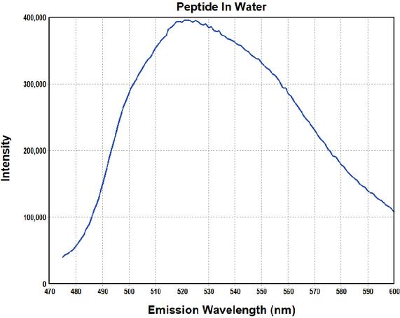
Figure 7 Fluorescence spectrum of the peptide with AuNPs in an aqueous solution.
Figure 8(a) shows the AFM image of the peptide deposited on a silicon wafer with a concentration of 86 M with AuNPs attached to the peptide fibers. In Figure 8(a) the lower left corner shows the fibers that have aggregated. The single fibers that can be seen in the images represent several -helices assembled into a linear fiber. The image was analysed with WSxM [25] and the average height of the fibers has been determined to be 3.0 nm 0.5 nm and the average height of AuNP peptide conjugates are 20.0 nm 0.5 nm, with the possibility of fibers underneath and above the AuNPs. The average distance between AuNP peptide conjugates were measured to be 453 nm. The theoretical calculated length of one -helix is around 3.5 nm, which means that there are between 90–100 -helices assembled between AuNPs. The dimers have been stabilised by the S-S bonds from cysteine bonds. The dimers formed longer fibers stabilised by hydrogen bonds. An estimate of the added number of AuNP have been calculated for both concentrations. For the concentration of 10 M, there are 100 AuNPs per peptide. For the concentration of 86 M, there are 12 AuNPs per peptide.
Figure 8(b) shows the peptide deposited on a Mica surface, at the same concentration as in Figure 8(a). Similar fibers can be seen on the mica surface as well, indicating that the fiber assembly is not induced by the surface properties. In both Figures 8(a) and 8(b) there are some fibers with AuNPs on, but there are also a few AuNP peptide conjugates present besides the fibers.
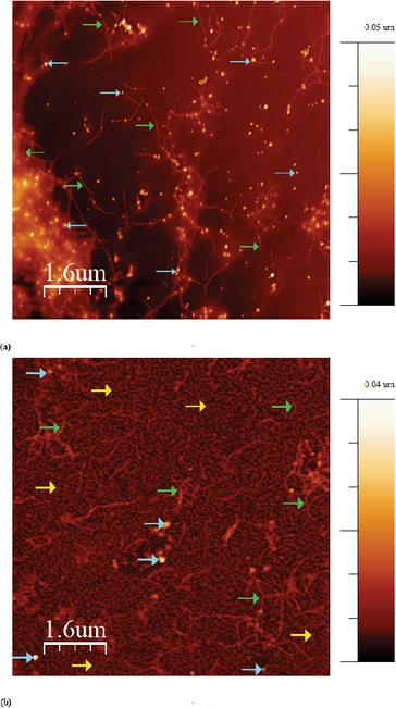
Figure 8 (a) AFM image of the produced peptide with AuNPs (blue arrows) on a silicon wafer with a peptide concentration of 86M (green arrows). (b) AFM image of the produced peptide with AuNPs (blue arrows) on a mica wafer (yellow arrows) with a peptide concentration of 86M (green arrows).
The AFM images, see Figures 9 and 8 show the designed peptide at different concentrations. The peptide concentration of 86 M shows long fibers with AuNPs bounded, while the AFM image for the peptide concentration of 10 M shows clumps of AuNP peptide conjugates, as a result of aggregation and islands of peptide almost enclosing some of AuNPs. For both concentrations, some of the AuNPs are bonded only to the surface and not to the peptide. This can be explained by the fact that the wafer surface is negatively charged and that the peptide has a limited number of cysteine residues for binding of AuNPS, resulting in the remaining AuNPs bind to the surface wafer instead of the peptide.
In Figure 9 the peptide concentration of 10 M on a mica wafer can be seen. It can be seen that the peptide aggregated into islands and single AuNPs randomly distributed on the surface. Comparing the 10 M concentration to the concentration of 86 M, the fiber formation is dependent on the concentration.
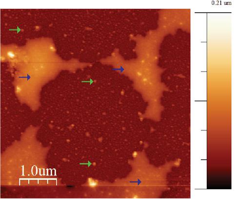
Figure 9 AFM image of the peptide at a concentration of (blue arrows) with AuNPs (green arrows) on a mica wafer.
The self-assembly process has been probed with MD simulations as well. For this purpose a simulation box containing water and the corresponding amount of peptide representing the same concentrations as the experimental concentrations has been generated. The MD simulations have been running at room temperature and the SASA has been followed to ensure sufficient simulation time, see Figure 10. This simulation was carried out for 800 ns. From this simulation, it can be seen that the SASA reaches a stabile value at 160 ns, indicating that the self-assembly is complete after this simulation time.
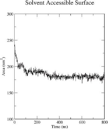
Figure 10 The SASA plot of the 86mM simulated peptide concentration.
The simulations have been running at higher peptide concentrations to ensure a faster assembly. Figure 11(a) shows the beginning of the simulation where the simulation box has the size 10 nm 5 nm 5 nm and contains 13 peptides. In the beginning of the simulation, the peptides were placed randomly as single peptides in the simulation box, and the system was neutralised with counter ions.
After 48 ns the peptides have assembled into fibers (Figure 11(b)). Subsequently, the fibers are stable and move within the simulation box. This corresponds well to the AFM images from Figure 8.
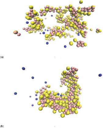
Figure 11 CG simulation with a box size of 10 nm 5 nm 5 nm containing 13 peptides. (a) Start of the CG simulation of the produced peptide with a concentration of 86 mM. (b) 48 ns of the CG simulation of the produced peptide with a peptide concentration of 86 mM. Here the peptides have assembled into fibers. The peptides are depicted as yellow and pink particles, and the blue particles are the ions added to keep the solution neutral during simulation.
For the concentration of 10 M a SASA plot was made to check when the simulation is saturated (Figure 12). This SASA plot was calculated from the MD simulation under the same conditions as the simulations for the concentration of 86 M, which were performed at room temperature. The simulation was carried out to 160 ns, where the graph begins to flatten at 150 ns, indicating that the simulation was saturated.
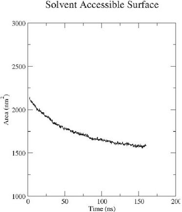
Figure 12 The SASA plot of the 10 mM simulated concentration.
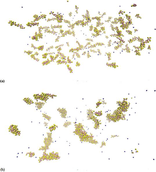
Figure 13 CG simulation with a box size of 40 nm 20 nm 20 nm containing 100 peptides. (a) Start of the CG simulation of the produced peptide with a concentration of 10 mM. (b) 94 ns of the CG simulation of the produced peptide with a concentration of 86 mM. Here the peptides are assembled into clumps. The peptides are depicted as yellow and pink particles, and the blue particles are the ions added to keep the solution neutral during simulation.
Figure 13(a) shows the beginning of the simulation with the simulation box of 40 nm 20 nm 20 nm containing 100 peptides. At the beginning of the simulation the peptides were separated into single helices with counter ions to keep the solution neutralised.
The simulation shows that the helices have assembled into small islands and thereby aggregated. This corresponds to the experimental data collected from the AFM images of Figure 9. This already happened at 94 ns in the simulation.
The observations in the AFM images correspond well with the CG simulations of the peptide, see Figure 8(b) and 11(b). In Figure 9 the peptide concentration of 10 mM can be seen, and the peptides assemble in islands with some AuNPs bonded, which fits the observed AFM image for the peptide concentration of 10 M, see Figure 9. The higher peptide concentration of 86 mM, as can be seen in Figure 11(b), also corresponds to the experimental observed AFM images, see Figure 8.
5 Copyright and Release Information
Permission is granted to quote short passages and reproduce figures and tables from ACES Journal issues provided the source is cited. Copies of ACES Journal articles may be made in accordance with usage permitted by Sections 107 or 108 of the U.S. Copyright Law. This consent does not extend to other kinds of copying, such as for general distribution, for advertising or promotional purposes, for creating new collective works, or for resale. The reproduction of multiple copies and the use of articles or extracts for commercial purposes require the consent of the author and specific permission from ACES.
6 Conclusion
The structure of the designed peptide has been predicted with both AlphaFold 1.5.2 [1] and PEP-FOLD 3.5 [2] to be an -helix. This was proven experimentally, and the helix is stable at room temperature. The ability of the peptide to bind stabile to AuNPs has been visually shown by AFM. In addition SPR were performed to confirm the binding of the peptide to Au surfaces. The incorporation of a fluorophore was verified. The AuNPs bound peptide with a fluorophore can assemble into long fibers and has a designed protease cleavage site, making this assembly a possible biosensor for protease activity.
Biographies
[1] M. Mirdita, K. Schütze, Y. Moriwaki, L. Heo, S. Ovchinnikov, and M. Steinegger, “ColabFold: makin protein folding accessible to all,” Nature Methods, vol. 19, pp. 679–682, 2022.
[2] P. T. A. Lamiable, J. Rey, M. Vavrusa, P. Derreumaux, and P. Tufféry, “PEP-FOLD3: faster de novo structure prediction for linear peptides in solution and in complex,” Nucleic acids research, vol. 44, pp. 499–454, 2016.
[3] R. Seyfi, F. A. Kahaki, T. Ebrahimi, S. Montazersaheb, S. Eyvazi, V. Babaeipour, and V. Tarhriz, “Antimicrobial Peptides (AMPs): Roles, Functions and Mechanism of Action,” International Journal of Peptide Research and Therapeutics, vol. 26, pp. 1451–1463, 2020.
[4] S. H. Snyder, “Brain Peptides as Neurotransmitters,” Science, vol. 209, pp. 976–983, 1980.
[5] R. S. Norton, “Enhancing the therapeutic potential of peptide toxins,” Expert Opinion on Drug Discovery, pp. 611–623, 2017.
[6] K. Reddy, R. Yedery, and C. Aranha, “Antimicrobial peptides: premises and promises,” International journal of antimicrobial agents, vol. 24, no. 6, pp. 536–547, 2004.
[7] J. Kopeček and J. Yang, “Peptide-directed self-assembly of hydrogels,” Acta biomaterialia, vol. 5, no. 3, pp. 805–816, 2009.
[8] E. Lin, C. H. Lin, and H. Y. Lane, “De Novo Peptide and Protein Design Using Generative Adversarial Networks: An Update,” Journal of chemical information and modeling, vol. 62, no. 4, pp. 761–774, 2022.
[9] A. P. McCloskey, B. F. Gilmore, and G. Laverty, “Evolution of Antimicrobial Peptides to Self-Assembled Peptides for Biomaterial Applications,” MDPI Open Access Journal, vol. 3, no. 4, pp. 791–821, 2014.
[10] P. Huang, S. E. Boyken, and D. Baker, “The coming of age of de novo protein design,” Springer Nature, vol. 537, no. 7620, pp. 320–327, 2016.
[11] H. Dong, S. E. Paramonov, and J. D. Hartgerink, “Self-Assembly of -Helical Coiled Coil Nanofibers,” Journal of the American Chemical Society, vol. 41, pp. 13691–13695, 2008.
[12] A. W. Senior, R. Evans, J. Jumper, J. Kirkpatrick, L. Sifre, T. Green, C. Qin, A. Žídek, A. W. R. Nelson, A. Bridgland, H. Penedones, S. Petersen, K. Simonyan, S. Crossan, P. Kohli, D. T. Jones, D. Silver, K. Kavukcuoglu, and D. Hassabis, “Improved protein structure prediction using potentials from deep learning,” Nature (London), vol. 577, no. 7792, pp. 706–710, 2020.
[13] J. Maupetit, P. Derreumaux, and P. Tuffery, “PEP-FOLD: an online resource for de novo peptide structure prediction,” Nucleic acids research, vol. 37, no. 2, pp. 498–503, 2009.
[14] B. Robson, “De novo protein folding on computers. Benefits and challenges,” Computers in biology and medicine, vol. 143, no. 105292, 2022.
[15] P. Thévenet, Y. Shen, J. Maupetit, F. Guyon, P. Derreumaux, and P. Tufféry, “PEP-FOLD: An updated de novo structure prediction server for both linear and disulfide bonded cyclic peptides,” Nucleic acids research, vol. 40, no. 1, pp. 288–293, 2012.
[16] M. Varadi, S. Anyango, M. Deshpande, S. Nair, C. Natassia, G. Yordanova, D. Yuan, O. Stroe, G. Wood, A. Laydon, A. Žídek, T. Green, K. Tunyasuvunakool, S. Petersen, J. Jumper, E. Clancy, R. Green, A. Vora, M. Lutfi, M. Figurnov, A. Cowie, N. Hobbs, P. Kohli, G. Kleywegt, E. Birney, D. Hassabis, and S. Velankar, “AlphaFold Protein Structure Database: massively expanding the structural coverage of protein-sequence space with high-accuracy models,” Nucleic acids research, vol. 50, no. D1, pp. 439–444, 2022.
[17] T. Hansson, C. Ostenbrink, and W. van Gunsteren, “Molecular Dynamics Simulations,” Current Opinion in Structural Biology, vol. 12, no. 2, pp. 190–196, 2002.
[18] J. Kreute, “Nanoparticles – a historical perspectives,” International Jonal of Pharmaceutics, 2007.
[19] V. J. Mohanraj and Y. Chen, “Nanoparticles – a review,” Tropical journal of pharmaceutical research, 2006.
[20] C. N. R. Rao, G. U. Kulkarni, P. J. Thomas, and P. P. Edwardsb, “Metal nanoparticles and their assemblies,” Chemical Society Reviews, 2000.
[21] A. J. Shnoudeh, I. Hamad, R. W. Abdo, L. Qadumii, A. Y. Jaber, H. S. Surchi, and S. Z. Alkelany, “Chapter 15 – Synthesis, Characterization, and Applications of Metal Nanoparticles, Biomaterials and Bionanotechnology,” Academic Press, 2019.
[22] A. Biswas, I. S. Bayer, A. S. Biris, T. Wang, E. Dervishi, and F. Faupel, “Advances in top–down and bottom–up surface nanofabrication: Techniques, applications future prospects,” Advances in Colloid and Interface Science, 2012.
[23] P. Suchomel, L. Kvitek, R. Prucek, A. Panacek, A. Halder, S. Vajda, and R. Zboril, “Simple size-controlled synthesis of Au nanoparticles and their size-dependent catalytic activity,” Scientific Reports, vol. 8, no. 4589, pp. 320–327, 2018.
[24] M. Oliveberg, S. Vuilleumier, and A. R. Fersht, “Thermodynamic Study of the Acid Denaturation of Barnase and Its Dependence on Ionic Strength: Evidence for Residual Electrostatic Interactions in the Acid/ Thermally Denatured State,” Biochemistry, vol. 33, pp. 8826–8832, 1994.
[25] I. Horcas, R. Fernández, J. Gómez-Rodríguez, J. Colchero, J. Gómez-Herrero, and A. Baró, “WSxM: A software for scanning probe microscopy and a tool for nanotechnology,” Review of Scientific Instruments, vol. 78, pp. 499–454, 2007.
[26] M. Abraham, T. Murtola, R. Schulz, S. Páll, J. Smith, B. Hess, and E. Lindahl, “GROMACS: High performance molecular simulations through multi-level parallelism from laptops to supercomputers,” SoftwareX, vol. 1–2, pp. 19–25, 2015.
[27] J. C. Phillips, D. J. Hardy, J. D. C. Maia, J. E. Stone, J. V. Ribeiro, R. C. Bernardi, R. Buch, G. Fiorin, J. Henin, W. Jiang, R. McGreevy, M. C. R. Melo, B. K. Radak, R. D. Skeel, A. Singharoy, Y. Wang, B. Roux, A. Aksimentiev, Z. Luthey-Schulten, L. V. Kale, K. Schulten, C. Chipot, and E. Tajkhorshid, “Scalable molecular dynamics on CPU and GPU architectures with NAMD,” Journal of Chemical Physics, vol. 153, 2020.
[28] W. Humphrey, A. Dalke, and K. Schulten, “VMD - Visual Molecular Dynamics,” Journal of Molecular Graphics, vol. 14, pp. 33–38, 1996.
[29] M. V. Kvach, D. A. Tsybulsky, A. V. Ustinov, I. A. Stepanova, S. L. Bondarev, S. V. Gontarev, V. A. Korshun, and V. V. Shmanai, “5(6)-Carboxyfluorescein Revisited: New Protecting Group, Separation of Isomers, and their Spectral Properties on Oligonucleotides,” Bioconjugate Chemistry, vol. 18, pp. 1691–1696, 2007.
Biographies

Julia Petersen received her Master’s degree in Nanomaterials and Nanophysics at Aalborg University, Department of Materials and Production in 2025. Her Master’s degree was pursued in the field of semiconductors. Currently she is pursuing a reaserch assistant position in planar magnetic components at Aalborg University, Department of Energy. Some of her research interests are biosensors, surface science, nanoparticles, and nanofabrication.

Katrine G. Eskildsen received her Master’s degree in Nanomaterials and Nanophysics from Aalborg University, Department of Materials and Production in 2025. Her research during her Bachelor’s and Master’s degrees included biosensor, surface science, nanoparticles, and nanofabrication. She is currently during her PhD studies in the Biophotonic Sensing Group at Lund University, Department of Combustion Physics, working on designing a LiDAR for diversity assessment of insects.
Journal of Self-Assembly and Molecular Electronics, Vol. 1_1, 1–22
doi: 10.13052/jsame2245-8824.111
© 2025 River Publishers